As any of you that used our two-enzyme GBS protocols know, the current GBS adapters are not set up for index reads – they were designed before Illumina introduced indexing. That is an issue when we want to pool those libraries with other indexed Illumina libraries; we always have to spend a bunch of time explaining the situation to the sequencing centres, and often end up having to do the demultiplexing ourselves.
No more! I have modified the adapters and primer designed so that you can get indexed GBS libraries, with adapters that are identical to standard TruSeq Illumina adapters (so they will work on any Illumina sequencer). The current “barcoded” adapters (PE1, i5) are actually fine, and you just need to use the indexed i5 primers we use for WGS libraries instead of the standard GBS PCR F primer. I had to re-design the Y-shaped “common” adapters (PE2, i7), as well as the corresponding primers. A list of all adapters, primers, in-line barcodes and indices is attached to the post.
Besides not having to worry about compatibility with other libraries when sequencing GBS libraries, adding indexes has of course the advantage of increasing the potential to multiplex GBS samples in a same lane. I kept the original 192 barcodes on the barcoded adapters and 12 barcodes on the common adapter; we already had 48 compatible indexed i5 primers, and I designed 24 indexed i7 primers – so you could potentially pool 192 * 12 * 48 *24 = 2,654,208 samples in a single lane. That’s probably not going to happen, but you can use the indices as an additional check to distinguish your libraries.
The barcoded adapters are still in Loren’s lab, but the rest of the adapters/primers are with me – just come and get them if you need them (my lab is in MSL385), or if you want to prepare your own aliquots.
Let’s face it, at some point of your research you will have
to grow some plants. It might seem overwhelming at first, especially deciding
on where and which facilities you should grow them in. Here is a small guide on
what is available.
Greenhouses
There are two main research greenhouses on campus:
Horticulture greenhouse and south campus research greenhouse.
Questions
to think about before selecting which greenhouse:
Is it indoor or outdoor?
How much security does my project require?
Easy access from campus?
What kind of environmental manipulation does you
need? Water, nutrient, lights, CO2?
How worry are you regarding pest? Preference on
pest control?
Does it require special treatment? Fertilizer
schedule?
Are you allergic to cats?
What is the minimum and maximum temperature I
will need?
Horticulture greenhouse
On campus, ~ 5 minutes walk from BRC
Glass greenhouse
Each compartment has its own irrigation tank
(compartment specific irrigation program possible)
Open roof vents (not screened)
Card access into building; alarm code for off
hour access
No CO2 manipulation (not equipped with CO2
emission)
Field site: totem field, ~ 5 minutes walk from
horticulture greenhouse
Has cats
South Campus Research Greenhouse
Near South campus ~ 30-minute walk, close to bus
stop
Isolated and gated facility
Key access
Closed roof vents (screened)
CO2 manipulation possible
Field site by the greenhouse
General irrigation (whole greenhouse irrigation;
no room specific tanks)
Polycarbonate greenhouse
Growth chamber
Bioscience building
Key access
Custom photoperiod, temperature. Humidity cannot
be modified
Limited walk-in chambers for tall plants (4 in
total)
More for growing low plants (Arabidopsis)
Need regular upkeep, measure light level before
starting your experiment
Internal space is limited
Limited pest control
Limited temperature range: from 15-40 degree.
The manual will tell you up to 45 but the wires used to maintain the growth
chambers can only tolerate 40 degrees.
Other departments have growth chambers that can
go down to low temperature (Forestry department).
Growth racks (in the lab)
For seedlings, or smaller plants. Not full size
sunflowers.
No temperature, humidity changes
Each rack has its own light. Photo period can be
adjusted using timers.
Limited space available
Perfect for Arabidopsis
I’ve decided on the space. Now what?
Once you’ve figured out where you want to grow your plants.
Here is the person to contact depending on what you want to use:
If anyone needs to design CAPS markers for genotyping based on SNP data, I wrote an R script to make the process of finding candidate SNPs in a large VCF much less painful.
I hosted it on RPubs in the form of a tutorial, which can be found here.
This article covers the steps needed to get to the point where you can run GATK commands on compute-canada. It will also provide recommendations on how to organize your files, achieve proper versioning, and request compute resources to run the command
as a precondition, you should:
have an account on compute canada
have a terminal/console application from which you can login to compute-canada, i.e. with ssh (either with password-based, or public-key based authentication)
We would suggest you also read other complementary articles on working with the terminal and command line tools, here (fixme update link).
For the purpose of this article, we’ll assume our goal is to produce an index file for a multi-GB VCF file.
There are many ways to do this. But GATK provides tool IndexFeatureFilefor this purpose. The tool will accept a VCF file as input (.vcf.gz), and produce a corresponding index file. (.vcf.gz.tbi).
There are other tools that can produce index files for gzipped VCF, namely a combination of bgzip and tabix. Most tools that produce indexes for vcfs produce files that are compatible with one another, but we’ll stick with the gatk brand for now.
We will cover the following steps to gatk properly on the compute cluster:
Login, and allocate a pseudo-terminal
Allocate/reserve a compute node
Load GATK (of the correct version)
from the compute-canada provided modules
from a “singularity” image
Launch the command. (we’ll cover the interactive way)
1 / Login and allocate a pseudo-terminal.
When you SSH into compute-canada, you are assigned a login node
In this case, I ended up on cedar5. If you don’t specify which login node you prefer, you’ll be assigned one randomly (by DNS). You can also specify the precise one you want, which comes in handy when one of them is unresponsive (or is being abused). You would state a preference by changing the hostname. There are two login nodes (as far as I’m aware) on the cedar cluster, cedar1 and cedar5. You can login to a specific one like so:
Now, we’re expecting our program to run for a while, so we’ll need to run it into a pseudo-terminal. Enter TMUX.
The program tmux buys us the ability to disconnect from cedar without interrupting the programs running on the terminal. It also allows us to run multiple interactive programs from the same terminal “window” and keyboard. It’s a way to “multiplex” our terminal window. I recommend tmux, because it has somewhat intuitive controls and comes with decent configuration out of the box, but you may prefer its competitor, screen.
You can create a new tmux-session, with the command:
# choose a meaningful name
$ tmux new-session -s gatk-stuff
Once it runs, it looks and feels just like a normal terminal, except there’s an extra bar at the bottom (in green), telling you you’re “one-level-deep” into virtual reality. A few new key combos will get recognized once you’re in tmux. Unlike in nested dreams, time doesn’t slow down as you go deeper, unfortunately.
The bar at the bottom tells you a few useful things, like the time, the server name, and the name of the session, i.e. [edit], in this case. You can run commands at the prompt like you would normally on a regular terminal emulator.
At some point you’ll want to “get out” of the tmux session. You can detach from the session with CTRL-B , followed by d. (d for “detach”). That’s control+b, release, then d. Then, you can re-attachto your named session with the command:
tmux attach-session -t gatkstuff
When your session is detached, the programs that you started are still running (they are not paused either. running). You can also disconnect completely from cedar, without affecting your detached session. Just make sure you detach from the session before exiting — typing exit inside a session will terminate the session, just as it would in a normal terminal window.
If you forget the name you gave your session, you may list them (here, 3):
[jslegare@cedar1 ~]$ tmux list-session
 edit: 1 windows (created Tue Feb 19 15:38:44 2019) 377x49
 gatk-stuff: 1 windows (created Wed Feb 20 13:10:57 2019) [80x23]
 run: 1 windows (created Tue Feb 19 15:34:25 2019) [271x70]#
I find that if I don’t touch a session for a while (generally 3-4 days), it will automatically be cleaned up. This happens when either the tmux server reboots, or cron reaps old processes on compute-canada. If you login and you don’t see your old session listed, it may be what happened. It may also be that the session was created on a different login node (cedar1 vs cedar5) — sessions are local to the server on which they were created.
CTRL-Bis the prefix to all tmux combos. That’s how you interact with the terminal. There are a lot of different ones to learn (https://gist.github.com/MohamedAlaa/2961058), but as you use them, they will make it to muscle memory. This is going to sound a little circular, but if you’re using an application which needs the key sequence CTRL-B for something, and you run that application inside tmux, you would send it the key combo CTRL-BCTRL-B. Some other useful combos are:
CTRL-B, ) Go to next session
CTRL-B, ( Go to previous session
CTRL-B, [ Enable scrolling mode. Scroll up and down with arrows, pageup/pagedown. Exit mode with Esc.
You can create “tabs” inside your tmux-sessions, which the tmux manual refers to as “windows”. And you can split the windows vertically and horizontally. You can also nest sessions, which is useful when your jobs involve multiple computers.
Note: It’s possible that your mouse wheel doesn’t quite feel the same when you’re inside tmux, depending on the version running. On some versions, “wheelscroll up” is interpreted as “arrow up”, which can be confusing. There’s a way to configure that, of course.
OK. before the next step, login to cedar, and create a new tmux session (or reattach to a previous one. We’re ready to run commands.
2/ Allocate a Compute Node
You can perform short program operations directly on the login nodes, but as a rule of thumb, any process that takes more than 10 cpu minutes to complete, or that consumes more than 4G of ram, should be run on a compute node that you have reserved. See Running Jobs.
To reserve a compute node, you would use one of the slurm commands, sbatchor salloc. The former will schedule a script to run, and run it in the background, eventually. The eventually is a big word which can mean anywhere from 10 seconds to 3 days. The latter, salloc,will allow you to interact directly with your reservation when it’s ready — it performs some terminal magic for you and places your job at the foreground in your terminal.
salloc is most useful when you’re experimenting with programs, like gatk in this case, and your work will involve a lot of trial and error. E.g. when you’re to nail down precisely which commands to add to your scripts. Another advantage of salloc over sbatchis that the node reservations you make sallocare considered “interactive”, and fall in a different wait queue of compute-canada. C-C reserves many nodes just for “interactive” work, so there is usually much less of a wait time to get your job running (usually 1min). However if you have 1000 instances of a script to run, sbatch will be the preferred way.
Example command to get an interactive node:
[jslegare@cedar1 test]$ salloc \
         --time 8:00:00 \
         --mem 4000M \
         -c 2 \
         --account my-account
 salloc: Granted job allocation 17388920
 salloc: Waiting for resource configuration
 salloc: Nodes cdr703 are ready for job
 [jslegare@cdr703 test]$ ... get to work ...
Time limit for the task: --time hh:mm:ss. Keep it under 24 h for interactive nodes.
CPUs: -c 2. The number of cpus (aka cores) to give to your task. This is the number of programs that can run “in parallel” simultaneously. Programs concurrently running share the available CPUs in time slices.
Memory: Memory--mem <N>G(GiB) or --mem <N>M(MiB). Total max memory in Gigabytes or Megabytes per task. This is dependent on the nature of the work you’ll do. 4Gwould be plenty for indexing a VCF. A rule of thumb is to give 2000M per cpu.
Account: --account my-account. This is how you choose which account will be billed for the utilization. Omit this parameter to see the list of accounts you can use. Not all accounts are equal, some will offer priority in the queues.
There are many more parameters you could use. Do man sallocto get the full list.
It is recommended that you specify the memory in megabytes, not gigabytes. If you ask for, e.g. 128G, you’re essentially asking for 131072M(128*1024M). Hardware nodes available which have a nominal 128GB of ram installed (and there’s a lot of them with this hardware config) won’t be able to satisfy a request for 128G(because some of it it reserved), but would be able to satisfy a request for 128000M.
Also, if you’re trying to have the queue on your side, you want to always be asking for fewer resources than everyone else — and the least amount possible that gets the job done. That’s a golden rule on c-c.
Once the salloc returns with satisfaction, you will get a shell prompt. Notice the hostname prefix changing on the command prompt, from cedar1(the login node), to cdr703(the compute node). The full address for compute nodes is:
<nodename>.int.cedar.computecanada.ca
This is useful to know because as long as you have a task running on a node, you can ssh into it, (by first hopping into cedar login nodes). This is true for jobs allocated both with sbatch, and salloc. You might need to have public key authentication setup for that to work however: compute nodes do not allow password login, as far as I know.
Logging in the compute node allows you to inspect the state of processes on that node while your task is running (e.g. with top), or inspect files local to the job
3 / Load GATK
We have an interactive node going, and now we’re ready to run some gatk commands. We need to modify our default paths to point to the particular gatkversion we want. I’m going to show two ways of doing it:
using the “modules” provided by compute-canada
using versions available online, in docker/singularity images.
Compute-canada, packages software in “modules” which can be added to the set of binaries you can run from the command line. In your environment you can load one version of gatk modules loaded at a time. It’s easy, but it’s not so convenient if you depend on different versions in the same script.
Method 1: using modules
To use GATK using slurm modules, you first need to:
At this point, the program gatkis on your PATH, and you can call it whichever way you like. The one thing to remember, is that the next time you open a session, you will have to load the module again.
Reproducibility: I highly recommend that you double-check the version of the gatk you are loading if you are depending on reproducibility. It’s hard to know when compute-canada staff may decide to change the version on you.
For instance, as a crude check in a script, you could add the following to ensure that gatk is there and its version is exactly 4.1.0.0. Six months from now, when you run your script again, you won’t have to remember which version you used:
My favourite method of running software that is version-sensitive, like GATK, is to not deal with slurm modules. I select the exact version of software I want from the web, and run it inside a singularity “container”. Think of a container as an archived and versioned ecosystem of files and programs. The authors of GATK publish tagged official versions of the software already installed in a minimal environment. All the gatk tools and the correct version of its dependencies (bash, perl, R, picard, etc.) are packaged together.
Other advantages are that it allows you to run multiple versions of gatk in the same session, and that it makes the software versions you need explicit in your scripts. Refer to this page for more info later: https://docs.computecanada.ca/wiki/Singularity
The list of GATK versions available to you are listed on docker hub, in the broadinstitute’s channel. Every new version of GATK will follow quickly with a new entry on the dockerhub channel.
You download a particular container of your choice (aka “pulling” a container), and then you run it:
[jslegare@cdr333 ~]$ singularity pull docker://broadinstitute/gatk:4.1.0.0
WARNING: pull for Docker Hub is not guaranteed to produce the
WARNING: same image on repeated pull. Use Singularity Registry
WARNING: (shub://) to pull exactly equivalent images.
Docker image path: index.docker.io/broadinstitute/gatk:4.1.0.0
Cache folder set to /home/jslegare/.singularity/docker
Importing: base Singularity environment
...
Exploding layer: sha256:6ce2cf3c2f791bd8bf40e0a351f9fc98f72c5d27a96bc356aeab1d8d3feef636.tar.gz
Exploding layer: sha256:2654b1d68e7ba4d6829fe7f254c69476194b1bdb0a6b92f506b21e2c9b86b1dc.tar.gz
WARNING: Building container as an unprivileged user. If you run this container as root
WARNING: it may be missing some functionality.
Building Singularity image...
Singularity container built: ./gatk-4.1.0.0.simg
Note the warning about reproducibility above. Technically the broadinstitute could overwrite the container with the tag 4.1.0.0 on the remote repository, which means you would be downloading a different container the next time around. But that would be extremely bad form. — akin to re-releasing new code under an old version. Some tags, like “latest” are meant to change. Others, with specific version numbers, are typically immutable, by convention.
more info about the goal here: https://www.ncbi.nlm.nih.gov/pmc/articles/PMC5706697/
Singularity saved the image (gatk-4.1.0.0.simg) in the same folder. These images are typically big (1-4GB), and they’re better off placed in a common location, for reuse.
Once you have the image, you have access to all the programs inside it:
[jslegare@cdr333 ~]$ singularity exec ./gatk-4.1.0.0.simg ls -ld /scratch/ ls: cannot access '/scratch/': No such file or directory
Notice however that the second command fails. This is because the container doesn’t contain a /scratchdirectory. If you wish to access a folder from the host computer from inside the container environment, you must use “bind mounts”.
[jslegare@cdr333 ~]$ singularity exec -B /scratch:/scratch ./gatk-4.1.0.0.simg ls -ld /scratch/
 drwxr-xr-x 20086 root root 1007616 Feb 28 23:17 /scratch/
The syntax is: -B <src>:<dst>. It makes directory or file <src> available at location <dst>inside the container environment. You can specify multiple -Bflags as well, for instance -B /scratch:/scratch -B /project:/project. But they need to be placed after the execkeyword, because they’re an option of the exec singularity subcommand. Also, your home folder /home/<user>/is mounted by default as a convenience, without having to specify anything.
If you’re not sure where programs are in a container, and you want to kick the tires, you can typically open an interactive shell session inside it (with bash, or ash, or sh):
[jslegare@cdr333 ~]$ singularity exec ./gatk-4.1.0.0.simg /bin/bash
 bash: /root/.bashrc: Permission denied
# inside the container
 jslegare@cdr333:/home/jslegare$ ls /home
 jslegare
 jslegare@cdr333:/home/jslegare$ ls /project
 ls: cannot access '/project': No such file or directory
 jslegare@cdr333:/home/jslegare$ which gatk
 /gatk/gatk
 jslegare@cdr333:/home/jslegare$ exit
 exit
# container is done. we're outside again
[jslegare@cdr333 ~]$ ls -ld /project
 drwxr-xr-x 6216 root root 675840 Feb 28 13:17 /project
Modifications to any files inside the container get reverted when the container exits. This lets your programs start fresh each time. But if you create new files inside a container, make sure they are placed in a folder that you have “bound” and is visibly accessible outside the container, such as your scratch or somewhere under your home folder. It’s also a good practice to mount the strict minimum number of folders needed to the container — it will limit the potential damage mistakes can do.
4/ Indexing a VCF
Ok, the hard part is done. Now we can index our VCF. GATK will have to read our entire VCF file, which come typically in .vcf.gzcompressed form, and then output the corresponding .vcf.gz.tbiin the same folder.
[jslegare@cedar1 my_vcf]$ pwd
 /scratch/jslegare/my_vcf
 [jslegare@cedar1 my_vcf]$ ls -lh
 -rw-rw-r-- 1 jslegare jslegare 14G Feb 28 16:56 my_file.vcf.gz
Above I’m showing you the vcf file. There are three things to notice:
It’s huge (14GB).
There is no accompanying index, which means that any vcf tool will take its sweet time to do anything with it.
it’s in my /scratch . this matters.
Placement tip 1: When we’re reading and writing large files, it’s faster to do it on a fast filesystem. If you have the choice, I recommend running the commands somewhere under /scratch/<myusername>/. Your /home/<myusername>and /project/foo/<myusername>will do, in a pinch, but they have higher-latency, smaller capacity, and they’re being constantly misused by hundreds of other users — which means they’re busy, to the point where they’re barely usable at all sometimes. That said, if the VCF you give is already somewhere outside /scratch/, it might not be worth your while to copy it to /scratch, and then move it back. But presumably, this is not the only command you’ll run on that VCF, so a copy might pay off eventually.
Placement tip 2: When you’re on a compute node (not the login node), there’s a special location that might even be faster than scratch, depending on your program’s access patterns. It’s a location that is backed by an SSD drive, local to the node. Whatever you store there is only visible inside that node, and it gets cleaned up when your task finishes or expires. It’s placed in the special variable: $SLURM_TMPDIR. You have about 100GB or so that you can use there, but you can ask for more in the sbatch or salloc command.
Placement tip 3: This is more advanced stuff, but if the disk is too slow for you, you can also create files and folders inside `/dev/shm`. The files you place there are backed by RAM, not the disk, and their total size count towards your job’s maximum memory allocation. In my experience however, gatk workloads don’t really benefit from that edge, because of the linear data formats. So stick with the previous two placement tips for basic gatk stuff, but keep this trick in your back pocket for your own tools.
Ok, the command we need is IndexFeatureFile, and we run it like so:
[jslegare@cdr333 my_vcf]$ singularity exec -B /scratch:/scratch docker://broadinstitute/gatk:4.1.0.0 gatk IndexFeatureFile -F my_file.vcf.gz
...
01:14:04.170 INFO  ProgressMeter - Ha412HOChr04:134636312              1.3                909000         677978.7
...
01:19:35.490 INFO  ProgressMeter - Ha412HOChr17:49367284              6.9               4672000         680776.7
01:19:54.254 INFO  IndexFeatureFile - Successfully wrote index to /scratch/jslegare/my_vcf/my_file.vcf.gz.tbi
 01:19:54.255 INFO  IndexFeatureFile - Shutting down engine
 [March 1, 2019 1:19:54 AM UTC] org.broadinstitute.hellbender.tools.IndexFeatureFile done. Elapsed time: 7.21 minutes.
 Runtime.totalMemory()=1912078336
 Tool returned:
 /scratch/jslegare/my_vcf/my_file.vcf.gz.tbi
That took 7.21 minutes to produce that tbi from a 14GB vcf.gz, and it claims to have needed 1.9GB of virtual memory to do it. A slight improvement to the basic command would be to give gatk a temp directory under $SLURM_TMPDIR, via the --tmp-dirargument. But insider gatk knowledge will reveal that this particular GATK command doesn’t cause much tempfile action.
Note: If you’ve loaded gatk with the slurm modules, then the only thing that changes is that you need to first runmodule load gatk. The command you run is then the same as above, without all the singularity command jazz.
Note 2: You may have noticed too that I ran singularity execon the full docker URL rather than the .simgfile you get from docker pull. It’s a bit slower than giving it the .simgbecause it has to “prepare” the image before it can run it. This involves downloading a few filesystem layers from the web (if it sees them for the first time), and copying things around. This process is accelerated if you link your singularity cache (~/.singularity/docker) to a location under /scratch/<username/.
It turns out that you can use half the amount of BigDye that is recommended by NAPS/SBC for Sanger sequencing and have no noticeable drop in sequence quality. The updated recipe for the working dilutions:
BigDye 3.1 stock 0.5 parts
BigDye buffer 1.5 parts
Water 1 part
I will prepare all future working dilutions using this recipe and put them in the usual box in the common -20ºC freezer. For more details on how to prepare a sequencing reaction see this post, and for how to purify them see this or this posts.
If you have several thousands of similar jobs to submit to a SLURM cluster such as Compute-Canada, one of your goals, aside from designing each job run as quickly as possible, will be to reduce the queuing delays — time spent waiting for an idle node to accept your job. Scheduling delays can quickly shadow the runtime of your job if you do not take care when requesting job resources — you may wait hours, or days even. One way to minimize waiting, of course, to schedule fewer jobs overall (e.g. by running more tasks within a given allocation if your allocation’s time is not expired). If you can fit everything in a single job, then perfect. But what if you could divide the experiment in two halves to run concurrently, thereby obtaining close to 200% speedup, and also spend less wallclock time in the job queue, waiting?
When working with compute tasks whose execution parameters can be moved along several different resource requirement axes (time, # threads, memory), the task of picking the right parameters can become difficult. Should I throw in more threads to save time? Should I use fewer threads to save ram? Should i divide the inputs into smaller chunks to stay within a time limit? Wait times are also, sometimes, multiplied if the jobs are resubmitted due to unforeseen errors (or change of parameters).
It helps to understand how the SLURM scheduler makes its decisions when picking the next job to run on a node. The process is not exactly transparent. The good news is that it’s not fully opaque either — There are hints available.
Selecting resources.
Once a job has been submitted via commands such as sbatch or srun, it will enter the job queue, along with the other thousands of jobs submitted by other fellow researchers. You can use squeue to see how far back you are in line, but that doesn’t tell you much. For instance, that will not always provide estimated start times.
You most likely already know that the amount of resources you request for your job, e.g. number of nodes, number of cpus, RAM, and wall-clock timelimit, have an influence on your job’s eligibility to run sooner. However, varying the amount of resources can have surprising effects on time spent in the scheduling state (aka state PENDING). The Kicker:
In some cases,increasingrequested job resources can lower overall queuing delays.
Compute nodes in the cluster have been statically partitioned by the admins. Varying the resource constraints of your job will change the set of of nodes available to run it somewhat similar to a step function. Each compute node on compute-canada (cedar and graham) is placed in one or more partitions:
cpubase_bycore (for jobs wanting a number of cores, but not all cores on a node)
cpubase_bynode (for jobs requesting all the cores on a node)
cpubase_interac (for interactive jobs e.g., `salloc`)
gpubase_… (for jobs requesting gpus)
etc.
If you request a number of nodes less than the number of cores available on the hardware, then your job request is waiting for an allocation in the _bycore partitions. If you request all of the cores available, then your job request will wait for an allocation in the _bynode partitions. So based on availability, it might help to ask for more threads, and configure your jobs to process more work at once. The SLURM settings will vary by cluster — the partitions above are for cedar and graham. Niagara, the new cluster, for instance, will only be doing by_node allocations.
On compute-canada: You can view the raw information about all available nodes and their partition with the sinfo command. You can also view the current node availability, by partition using partition-stats.
The following command outputs a table that shows the current number of queued jobs in each partition. If you look in the table closely, you learn that there is only one job in the queue for any node in the _bynode partition (for jobs needing less than 3 hours). The _bycore partition, on the other hand, has a lot of jobs sitting on it patiently. If you tweak your job to make it eligible for the partition with the most availability (often it is the one with the most strict requirements), then you minimize your queuing times.
$ partition-stats -q

     Number of Queued Jobs by partition Type (by node:by core)

Node type | Max walltime
          | 3 hr  | 12 hr   | 24 hr   | 72 hr  | 168 hr | 672 hr  |
----------|--------------------------------------------------------
Regular   | 1:263 | 429:889 | 138:444 | 91:3030| 14:127 | 122:138 |
Large Mem | 0:0   | 0:0     | 0:0     | 0:6    | 0:125  | 0:0     |
GPU       | 6:63  | 48:87   | 3:3     | 8:22   | 2:30   | 8:1     |
GPU Large | 1:-   | 0:-     | 0:-     | 0:-    | 1:-    | 0:-     |
----------|--------------------------------------------------------
“How do I request a _bynode partitioning instead of a _bycore ?”
That is not obvious, and quasi undocumented. The answer is that you do so by asking for all the cpus available on the node. This is done with sbatch --cpus-per-task N. To get the best number of CPUs N, you have to dig a bit deeper and look at the inventory (this is where the sinfo command comes handy). The next section covers this. And this is something that may change over time as the cluster gets upgrades and reconfigurations.
Also, if you request more than one node in your job, each with N CPUs (e.g. sbatch --nodes=3 --cpus-per-task=32 ...), then all of them will be _bynode.
Rules of Thumb
Here are some quick rules of thumb which work well for the state of the cedar cluster, as of April 2018. The info presented in this section was gathered with sinfo, through conversations with compute-canada support, and through experience (over the course of a few weeks). In other words, I haven’t attempted to systematically study job wait times over the course of months, but I will claim that those settings have worked the best so far for my use cases (backed with recommendations from the support team).
Most compute nodes have 32 CPUs installed. If you sbatch for N=32 cpus --cpus-per-task=32, you are likely to get your job running faster than if you ask for, say N=16 cpus. If your job requires a low-number of CPUs, then it might be worth exploring options where 32 such jobs are run in parallel. It’s okay to ask for more, but try to use all the resources you ask for, since your account will be debited for them.
Most compute nodes have 128G ram. If you keep your job’s memory ceiling under that, you’re hitting a sweet spot. You’ll skip a lot of the queue that way. Next brackets up are (48core, 192G) (half as many as in the 128G variety), and (32 core, 256G) (even fewer).
Watch out for the --exclusive=userflag. The flag --exclusive=user tells the scheduler that you wish your job to only be colocated with jobs run by your user. This is perhaps counter-intuitive, but it does not impose a _bynoderestriction. In the case where your job is determined to be _bynode(i.e., you request enough cpus to take a whole node), this flag is redundant. If you don’t ask for all cores available (meaning your job needs a _bycore allocation), then this flag will prevent jobs from other users from running on that node (on the remaining cpus). In that case, the flag will likely hurt your progress (unless you have many such jobs that can fill that node).
The time limit you pick matters. Try to batch your work in <= 3H chunks. A considerable number of nodes will only execute (or favor) tasks which can complete in less than 3H of wallclock time. There’s a considerable larger amount of nodes that will be eligible to you also if you go under the 3H wallclock time limit. The next ‘brackets’ are 12H, then 24H, 72H, 168H (1 wk), and 28d. This suggests that there is no benefit to asking for 1H vs 3H, or 22H vs 18H, although an intimate conversation with the scheduler’s code would confirm that.
But, I want it now.
It should be mentioned that often, if only a single “last-minute” job needs to be run, salloc (same arguments as sbatch, mostly) can provide the quickest turnaround time to start executing a job. It will get you an interactive shell to a node of the requested size within a few minutes of asking for it. There is a separate partition, cpubase_interac, which answers those requests. Again, it is worth looking at the available configurations. Keep salloc it in your back pocket.
We already have a GBS protocol on the lab blog, but since it contains three different variants (Kate’s, Brook’s and mine) it can be a bit messy to follow. Possibly because I am the only surviving member of the original trio of authors of the protocol, the approach I used seems to have become the standard in the lab, and Ivana was kind enough to distill it into a standalone protocol and add some additional notes and tips. Here it is!
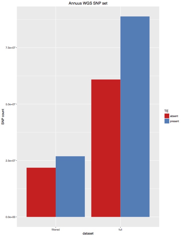
I’ve often wondered if the TEs in the sunflower genome were producing erroneous SNPs. I have unintentionally produced a little test of this. When calling SNPs for 343 H. annuus WGS samples I set FreeBayes to only call variants in non-TE parts of the genome (as per our TE annotations). Unfortunately, I coded those regions wrong, and actually called about 50% TE regions and 50% non-TE regions. That first set was practically unfiltered, although only SNPs were kept. I then filtered that set to select high quality SNPs (“AB > 0.4 & AB < 0.6 & MQM > 40 & AC > 2 & AN > 343 genotypes filtered with: DP > 2”). For each of these, I then went back in and removed SNPs from TE regions, and I’ve plotted totals below:
There are a few things we can take from this:
There are fewer SNPs in TE regions than non-TE regions. Even though the original set was about 50/50, about 70% of SNPs were from the non-TE regions.
For high quality SNPs, this bias is increased. 80% of the filtered SNPs were from non-TE regions.
Overall, I think this suggests that the plan to only call SNPs in non-TE regions is supported by the data. This has the advantage of reducing the genome from 3.5GB to 1.1GB, saving a bunch of computing time.
When you get your GBS data from the sequencer, all your samples will be together in one file. The first step is to pull out the reads for individual samples using your barcodes. There are many ways of doing this, but here is one.
3rd generation sequencing technologies (PacBio, Oxford Nanopore) can produce reads that are several tens of Kb long. That is awesome, but it means that you also need to start from intact DNA molecules of at least that size. I thought the DNA extraction method I normally use for sunflower would be good enough, but that is not the case. Continue reading →
This is a protocol Allan DeBono used when cleaning BigDye 3.1 sequencing reactions for sequencing at NAPS. In both of our hands it worked consistently to confirm vector inserts. An advantage for this protocol is that it takes 5-10 minutes to preform depending on how many reactions are being run (and how fast of a pipetter you are). It also utilizes spin columns that can be re-used after autoclaving. Continue reading →
NAPS, the UBC service we use for Sanger sequencing, charges 2 CAD for purifying a sequencing reaction; especially if submitting several reactions, there is therefore a reasonably big incentive in doing the purification ourselves. Continue reading →
Since I started in the lab, I had the impression that the SB buffer we use for gel electrophoresis did not work quite as well as the more commonly used TAE buffer, but as I wasn’t running many gels I was too lazy to run a test. Also, Wikipedia said I was wrong, and who am I to doubt Wikipedia?
Argophyllus has a reputation of being a plant it is hard to get DNA from. As a test for a larger project, I did a round of extractions from annuus, petiolaris and argophyllus. I used the modified 3% CTAB method I described before, starting from one fresh, frozen, very young (~1-2 cm long) leaf.
For all species, the CTAB extraction yielded about 50 µl of 200-500 ng/µl solution (10-25 µg in total) of clean (260/230 = 2.05-2.20) genomic DNA, with minimal shearing (see picture). Continue reading →
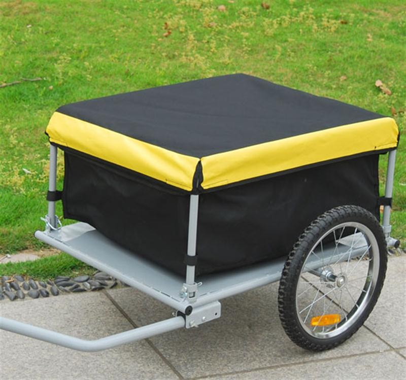
This is just to let everybody know that for those that are working around campus this summer, we have a bike trailer that can be helpful to transport small equipment or a bunch of plants from the lab to the greenhouse, Totem field or anywhere near by. There is also a lock for it and hopefully, and most importantly we will soon have an additional bike apart from the rusty one that Brook kindly donated some time ago. I will keep you updated on that!
Share and enjoy! (make sure to always return it to the lab so it’s available for the rest of us)
There is a version of the GBS barcode protocol that has barcodes on both adapters. Although scripts existed for demultiplexing dual enzyme GBS (including PyRad and Stacks), it didn’t seem like any of them let you demultiplex for dual barcodes. For this you need you need to determine the sample identity by both barcodes (i.e. either barcode may not be unique) and you need to strip out barcode sequence.
If you are interested by generating quickly a list of compounds that were previously identified in a plant, the online dictionary of natural product is a good place where to start your research. It regroups entries for >270k natural chemical compounds.
In the current version of the website (March 2016) you can search for “Biological source” and in there “the latin name of your favourite species”. The result of such a query for “Helianthus” is a list of 381 chemical compounds that were tagged as identified in Sunflower species (and a minority of other species with helianthus in the name). Of course this list is quite restricted compared to the number of metabolites produced by sunflower plants. It is however a good starting point to know what kind of compounds (here a lot of terpenes, few flavonoids) were previously extracted from your favourite plant species. Some entries are tissue specific, such as large terpenes from pollen. Also interesting, the “biological use” column gives sometimes information on the role of the compound (e.g. antifungal, allelochemical, growth inhibition).
The CAS registry number is probably the most powerful piece of information you can get out of such a search. It’s the unique ID for the compound and can be use to search the compound in multiple databases. My favourite are:
Chemspider: This is probably the more powerful chemical database that currently exists. It’s huge: it regroups information for more than 44 million chemical structure and cross-reference with many other databases.
Pubchem: It will look really familiar to NCBI/pubmed users. With pubchem you can for exemple submit the CAS number and get a list of publications linked to the compound.
When analyzing genomic data, we first need to align to the genome. There are a lot of possible choices in this, including BWA (medium choice), stampy (very accurate) and bowtie2 (very fast). Recently a new aligner came out, NextGenMap. It claims to be both faster and deal with divergent read data better than other methods. Continue reading →