The good news: it looks like PstI-MspI GBS offers substantial benefits over PstI alone, even without depleting high copy fragments. Marco’s DSN protocol may improve things further, and we have a trial sequencing library running now.
Tag Archives: SNP
GBS, coverage and heterozygosity. Part 3
I’ve recalled the SNPs for my Helianthus exilis population genetics for a third time. This time I’m using GATK. This is aligned using BWA to the Nov22k22 reference.
This is two plates of GBS (96-plex each) plus 34 H. annuus samples from G. Baute (also 96-plex GBS). Three exilis samples were removed because they had little or no reads. Reads were trimmed for adapters and quality using trimmomatic (and the number of reads kept after trimming are used here).
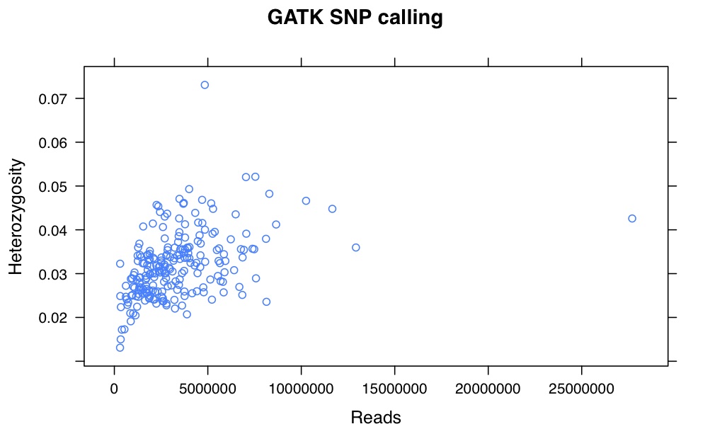
So, there is a relationship between number of reads and resulting heterozygosity. It makes some sense because you need a higher number of reads to call a heterozygote than a homozygote. It’s not as bad as what was happening when we were calling snps using the maximum likelihood script. Using a linear model, number of reads accounts for %16 of the variation in heterozygosity.
If you compare this to my previous posts, the heterozygosity is vastly lower for all samples. That is because I previously looked at variable sites with a certain amount of coverage, and here are all sites. So a majority of these sites are invariant.
GBS snp calling
One of the main ways we call SNPs in GBS data is using a maximum likelihood script derived from the original Hohenlohe stickleback RAD paper. It uses a likelihood function based on the number of reads for each base at a site to determine if its homozygous or heterozygous.
It’s been known for a while that it seemed to be biased against high coverage heterozygous sites. I took the script apart and realized that there was actually a serious problem with it. The likelihood function used factorials, and when there were over 175 reads at a site, perl broke down and started describing things as infinite. Then the script would call it as a homozygote by default.
Letting perl work with the huge numbers necessary makes it incredibly slow, so I put in a logic gate for high coverage sites. If there is over 150 reads at a site, and the second most numerous base makes up atleast 10% of the reads (i.e. at minimum 15), then it is heterozygous. Otherwise it is homozygous.
The rest of the script is the same. One could debate how best to call the high coverage scripts, but I suggest you use this script over the old one.
Filtering SNP tables
Previously I posted a pipeline for processing GBS data. At the end of the pipeline, there was a step where the loci were filtered for coverage and heterozygosity. How strict that filtering was could be changed, but it wasn’t obvious in the script and it was slow to rerun. I wrote a new script that takes a raw SNP table (with all sites, including ones with only one individual called) and calculates the stats for each loci. It is then simple and fast to use awk to filter this table for your individual needs. The only filtering the base script does is not print out sites that have four different bases called at the site.
Heterozygosity, read counts and GBS: PART 2
Subtitle: This time… its correlated.
Previously I showed that with the default ML snp calling on GBS data, heterozygosity was higher with high and low amounts of data. I then took my data, fed it through a snp-recaller which looks for sites that were called as homozygous but had at least 5 reads that matched another possible base at that position (i.e. a base that had been called there in another sample). I pulled all that data together, and put it into a single table with all samples where I filtered by:
AWK unlinked SNP subsampling
For some analyses, like STRUCTURE, you often want unlinked SNPs. For my GBS data I ended up with from 1 to 10 loci on each contig which I wanted to subsample down to just one random loci per contig. It took me a while to figure out how to do this, so here is the script for everyone to use:
cat YOUR_SNP_TABLE | perl -MList::Util=shuffle -e ‘print shuffle(<STDIN>);’ | awk ‘! ( $1 in a ) {a[$1] ; print}’ | sort > SUBSAMPLED_SNP_TABLE
It takes you snp table, shuffles the rows using perl, filters out one unique row per contig using awk, then sorts it back into order. For my data, the first column is CHROM for the first row and then scaffold###### for the subsequent rows so the sort will place the CHROM row back on top. It might not for yours if you have different labels.
Scripts for Formatting SNP Tables
Some SNP table to useful table conversion scripts are here: FormattingScripts_v0.4
Readme.txt explains usage, makes fasta, bayescan, structure files as well as converting to digits for R.
Let me know if you find any of this useful or broken.
Greg
Edit: updated small fix to structure formatter
Jaatha – training data sets (Rose)
I’ve generated three training data sets, which will save you around 5 days if you decide to run Jaatha, a molecular demography program. It uses the joint site frequency spectrum of two populations to model various aspects of population history (split time, population size and growth, migration). Here’s the paper: Naduvilezhath et al 2011.
1. Using the default model, with the following maxima: tmax=20, mmax=5, qmax=10.
2. Alternative maxima: tmax=5, mmax=20, qmax=20.
3. Alternative maxima: tmax=5, mmax=20, qmax=5.
They can’t be uploaded because they’re compressed R data structures, but let me know if you’d like to give them a whirl.
Turning your SNP table into a STRUCTURE input file (Brook)
 I suspect there are probably several homemade versions of this kind of script kicking around, but here is a perl script I’ve written for turning your SNP table into a STRUCTURE input file. To use it, you should change the .txt to a .pl after downloading the script. More on STRUCTURE input files (and so much more!) is in the documentation here.
Merge SNP calls (Greg B.)
Rose coded this up as a faster and efficient way to combine all the snp calls into one table. I’ve made a few modifications, hopefully its not broken. Updates are likely in the future.
SNP calling with ML (Greg B.)
Email for v7. Bug found that printed G’s as C’s and vise versa.
Call SNPs from sam files in a method similar to Hohenlohe et al 2010. Updated to v4 Feb 9. Previous version had a bug.
It is now fixed up for all of BWAs cigars flavors.
This only deals with reads that fit one of the following:
Full alignment (55M)
Soft clip at the start (10S45M)
Soft clip at end (45M10S)
One deletion (25M10D25M)
One insertion (20M10I20M)
This means it ignores reads with a cigar fields that have N, H, P, = or X and it ignores reads with a cigar more complicate then a single soft clip or a single indel. It also does not penalize reads adjacent to indels.
It ignores bases in soft clipped parts of reads
SNP table parsing (Greg B.)
Ask me for the most current version if you want to use any of these!
A few perl scripts that take a SNP table and do the following:
1. Remove unwanted samples and rename the samples
2. Remove sites that do not have enough data
3. Order the sites based on a map
Population Genomics! (Greg B.)
Ask me for the most current version of these if you want to use them.
Several people in the lab are now working with very similar data (in structure) and have similar questions (in technique). As I have discussed with several people it would be very useful if we could all build up and share the tools needed to do these analysis. Understandably, people may want to do things on their own or in a specific manner, but I think there are several advantages to building this up together. The main thing is that it will be more efficient in terms of personnel time, having each person re-invent the wheel does not make sense. I think the blog is a great place to set do this. Below we can make our wish list and link to posts for solutions as they become available. As always, the principles (1,2 and 3) covered here apply.
SNP summary statistics in R: ‘hierfstat’ is back and better than before! (Rose)
After being disabled and not supported for several months, ‘hierfstat’ (by Jerome Goudet) now has lots of useful (and fast) calculations of summary statistics, including expected and observed heterozygosity, Fst and Jost’s Dest.