Purging GBS index switching

Quote

Considering the amount of sequencing coming out of the newer Illumina machines, we’ve started to combine GBS libraries with other samples. Due to how GBS libraries are made, when multiplexed with whole genome sequencing samples, there is an appreciable amount of contamination from GBS to WGS. That means you will find GBS reads in your WGS data. I’ve quantified that in the following figure, showing the percent of barcoded reads in WGS samples.

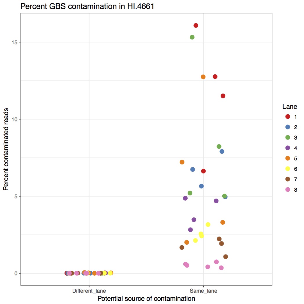
The left side is contamination from barcodes sequenced in different lanes (i.e. ones where they couldn’t contaminate). The right side is barcodes from GBS samples sharing the same lane (i.e. ones that could contaminate. The take home message is that between 1% to 15% of reads are GBS contamination. This is far above what we want to accept so they should be removed.

I’ve written a script to purge barcoded reads from samples. You give it the set of possible barcodes, both forward and reverse (All current barcodes listed here: GBS_2enzyme_barcodes). I’ve been conservative and been giving it all possible barcodes, but you could also trim it to only the barcodes that would be present in the lane. It looks for reads that start with the barcode (or any sequence 1bp away from the barcode to account for sequencing error) plus the cut site. If it finds a barcoded read, it removes both directions of reads. It outputs some stats at the end to STDERR. Note, this was written for 2-enzyme PstI-MspI GBS, although could be rewritten for other combinations.

An example of how you could apply this:

Make a bash script to run the perl script:

input=$1
perl ../purge_GBS_contamination.pl /home/gowens/bin/GBS_2enzyme_barcodes.txt ${input}_R1.fastq.gz ${input}_R2.fastq.gz ${input}.tmp;
gzip ${input}.tmp_R*.fastq

Run this bash script using gnu parallel

ls | grep .gz$ | grep R1 | sed s/_R1.fastq.gz//g | parallel -j 10 bash .decontaminate.sh 2>> decontamination_log.txt


Filtering TEs from SNP sets

I’ve often wondered if the TEs in the sunflower genome were producing erroneous SNPs. I have unintentionally produced a little test of this. When calling SNPs for 343 H. annuus WGS samples I set FreeBayes to only call variants in non-TE parts of the genome (as per our TE annotations). Unfortunately, I coded those regions wrong, and actually called about 50% TE regions and 50% non-TE regions. That first set was practically unfiltered, although only SNPs were kept. I then filtered that set to select high quality SNPs (“AB > 0.4 & AB < 0.6 & MQM > 40 & AC > 2 & AN > 343 genotypes filtered with: DP > 2”). For each of these, I then went back in and removed SNPs from TE regions, and I’ve plotted totals below:

There are a few things we can take from this:

  • There are fewer SNPs in TE regions than non-TE regions. Even though the original set was about 50/50, about 70% of SNPs were from the non-TE regions.
  • For high quality SNPs, this bias is increased. 80% of the filtered SNPs were from non-TE regions.

Overall, I think this suggests that the plan to only call SNPs in non-TE regions is supported by the data. This has the advantage of reducing the genome from 3.5GB to 1.1GB, saving a bunch of computing time.

GBS dual-barcode deplexer

There is a version of the GBS barcode protocol that has barcodes on both adapters.  Although scripts existed for demultiplexing dual enzyme GBS (including PyRad and Stacks), it didn’t seem like any of them let you demultiplex for dual barcodes. For this you need you need to determine the sample identity by both barcodes (i.e. either barcode may not be unique) and you need to strip out barcode sequence.

Continue reading

Comparing aligners

When analyzing genomic data, we first need to align to the genome. There are a lot of possible choices in this, including BWA (medium choice), stampy (very accurate) and bowtie2 (very fast). Recently a new aligner came out, NextGenMap. It claims to be both faster and deal with divergent read data better than other methods. Continue reading

Splits tree and iupac coding

I’ve been running splitstree to see the relationships between samples of H. bolanderi. I have coded my data using IUPAC so hets are a different symbol (Y, W, etc). The other way to code heterozygous sites into fasta is just pick one allele randomly.

By default, splitstree ignores all ambiguous sites, so if you use IUPAC coding, it will ignore all those sites. I switched it from ignoring, to using an average for all possible alleles. This made my tree much messier and had a weird smattering of samples pulled toward the outgroup. I’ve figured out that it has to do with the amount of missing data. Since Ns are ambiguous, when you average N it just sort of homogenizes the distances between samples. Thus, it can pull your samples into weird positions if they have different amounts of missing data.

My thoughts are that you should just ignore ambiguous data if you have enough sites to resolve your samples without them.

Sample Information Table

There is a constant problem of record keeping in the lab, and it is the most annoying in regards to sequence data. We have lots of data but finding out exactly what plants the data came from is difficult. So, I’m taking the old sample information table Seb made years ago and making it mandatory.

You must fill out this form before you get access to your sequence data. There will be one row per sample, meaning that for a GBS library you will have 96 or 192 rows.

Sample information table

Need cM positions?

Hello,

For a lot of work, it is helpful to know the cM position of your snps. Here is a script that takes the linkage map produced by Chris, your snp table in Hapmap format, and adds a column giving you a cM position for each site. It interpolates between known positions, so individual positions the accuracy of the position is overstated, but it’s good for plotting.

https://github.com/owensgl/reformat/blob/master/hmp2cmpositions.pl

usage:

perl hmp2cmpositions.pl /moonriseNFS/HA412/pseudomolecules/lg.ALL.bronze14.path.txt yoursnptable.hmp > yoursnptable.withcm.hmp


Phred score detector

When using old sequence data you have to know what phred score system it is using. Almost all new data is going to use Phred33, but the old stuff could also be Phred64. There are scripts on this website that have ways of automatically detecting it http://wiki.bits.vib.be/index.php/Identify_the_Phred_scale_of_quality_scores_used_in_fastQ

I took the perl script from this website and parred down the output so that it works in pipelines. It outputs either “phred33” or “phred64”

fastq_detect_minimal.pl

An example pipeline in bash is:

coding=”$(perl $bin/fastq_detect_minimal.pl ${name}_1.fq)”

java -jar trimmmomatic-0.32.jar -$coding sample1.fq ….etc

NOTE: Phred64 should only go up to 104. There are some RNA seq samples (and probably others) that go up to 105. The original script output an error, while my version just says phred64. I hope that running it through phred conversion in trimmomatic fixes the issue but I am not sure.

Percent reads aligned collector

When you publish next gen sequencing data you have to include the percent reads aligned. The number is easy to get but when you have 200+ samples it’s a pain to collate them together. This script takes a directory with bam files, uses samtools flagstat to get percent reads aligned and then does a little rejiggering of format to put it in a nice list. To run it, enter the directory with the bams and type ‘bash ./percent_counter.bash’

percent_counter.bash NOTE: The script is gzipped.

GBS barcodes 1-96 stocks

In the freezer there is a deep well plate with annealed barcodes 1-96, labelled plate 1C. Recently Dan Bock and myself used it to make stock concentration plates. Plate 1C has been qubit three times, here is an excel spreadsheet with the concentrations. They are in chronological order (i.e. Dan’s measurements are the most recent). I’ve also included an average column.

qubit-1-96GBS

So if you need to make your own plates for barcodes 1-96, you can use this. Dan Bock recommends diluting to a 4X concentration, qubiting that plate, then using that to dilute to 1X concentration if you want to be more accurate.

The limits of GBS sample size

Image

I’ve been doing work on a stickleback GBS dataset and we’re trying to figure out how many samples we can cram into a single lane of illumina. I did some analyses which people may find useful. It’s unclear how applicable the recommendations are for sunflower which seems to have more problems than fish.

Take home message, with 25% less data you lose around 15% of the genotype calls, but up to 50% of the SNPs if you use a stringent coverage filter, due to how the lost data is distributed among loci and individuals.

SNP calling with GATK warning

I’ve come to the realization that I’ve been making a mistake in my SNP calling using GATK. I’ve been filtering for site quality not for individual genotype quality. This is a critical difference and leads to some dubious SNPs being called.

It works like this. For each position in the genome, GATK will use all the data together to call whether an alternate allele exists. This is represented by the phred scaled QUAL score. A high QUAL score means that the alternate allele exists in in your dataset. This number is often very high if you’re analyzing a whole plate of GBS because it takes into account all the data from all the individuals. I’ve been filtering based on this number.

There is also a MQ score, which is the mapping quality for all the reads at that site.

For each individual, if there are any reads at that site GATK will output a genotype call (i.e. 0/0, 0/1, 1/1). It also outputs the number of reads supporting each allele, the QT score (which is the phred scaled probability of that the genotype call being correct) and the likelihoods of each possible genotype. When you use select variants in GATK, it filters sites but not genotypes (so you can have a site that is good, but individual genotype calls at that site that are bad).

If you use vcf-to-tab to convert your vcf to tab separated it will accept every genotype call. This means that for some individuals you will have 1 read supporting the reference and it will be called as 0/0. The QT score will be 3, which is incredibly low, but vcf-to-tab ignores that information and calls it. Therefore a proportion of your SNPs are highly questionable. This likely contributes to the heterozygote loss seen in GBS data.

Sam and Chris wrote a script that converts a vcf file to tab but also makes sure that the quality (QUAL, QT, MQ, and depth) is good. I’ll post it if they’re OK with it be up.

Edit: Here are the scripts. They are identical except one outputs in IUPAC format (AT=W, AC=M, etc) and the other outputs in the standard double nucleotide format (AA, AT, etc).vcf2vertical_dep_GATK-UG vcf2vertical_dep_GATK

Also note that sometimes GATK will output a genotype call that looks like:

./.:.:3

While normally they should look like:

./. or 0/0:17,0:18:45:0,45,353

This is saying that there are three reads at this position, but the quality is so bad that GATK is not calling the genotype. If you have these, the scripts will throw an error but will correctly output an NN for that genotype. So if you get a normal output and many errors, it’s probably OK.

FTP to a server

If you want to download something from a sequence read archive, often the files are available on ftp. A browser will automatically download those ftp files if you click the link, but if you are working on a server, it is a pain to download the file to your home computer and then upload it. Here is a quick guide to do this on the command line.

1)Copy the link address for the ftp file you want, from the website.

ftp://ftp.sra.ebi.ac.uk/vol1/fastq/ERR168/ERR168678/ERR168678_2.fastq.gz

2) SSH to your server and navigate to the folder your want to put the data in.

3) Type ‘ftp’. You are now in the ftp prompt.

ftp

4) Open a connection to the ftp server by typing in ‘open <server name>’. It asks you for a name, and if you don’t have one try ‘anonymous’. It asks for a password, try just pressing enter.

ftp> open ftp.sra.ebi.ac.uk
Connected to ftp.sra.ebi.ac.uk.
220-
220- ftp.era.ebi.ac.uk FTP server
220
Name (ftp.sra.ebi.ac.uk:owens): anonymous
331 Please specify the password.
Password:
230 Login successful.
Remote system type is UNIX.
Using binary mode to transfer files.

5) Navigate to the file you want using ‘cd’ to change directory and ‘ls’ to view directory contents.

ftp> cd vol1/fastq/ERR168/ERR168678
250 Directory successfully changed.
ftp> ls
200 PORT command successful. Consider using PASV.
150 Here comes the directory listing.
-r–r–r– 1 ftp ftp 10990053136 Dec 22 2012 ERR168678_1.fastq.gz
-r–r–r– 1 ftp ftp 10998002687 Dec 22 2012 ERR168678_2.fastq.gz
226 Directory send OK.

6) Download data using ‘get <filename>’

get ERR168678_2.fastq.gz

7) Your data is now downloading. Its best to run this in a screen so that you don’t have to keep the window open, in case it runs slowly.

GBS, coverage and heterozygosity. Part 3

I’ve recalled the SNPs for my Helianthus exilis population genetics for a third time. This time I’m using GATK. This is aligned using BWA to the Nov22k22 reference.

This is two plates of GBS (96-plex each) plus 34 H. annuus samples from G. Baute (also 96-plex GBS). Three exilis samples were removed because they had little or no reads. Reads were trimmed for adapters and quality using trimmomatic (and the number of  reads kept after trimming are used here).

Exil.GATK.file.het


So, there is a relationship between number of reads and resulting heterozygosity. It makes some sense because you need a higher number of reads to call a heterozygote than a homozygote. It’s not as bad as what was happening when we were calling snps using the maximum likelihood script. Using a linear model, number of reads accounts for %16 of the variation in heterozygosity.

If you compare this to my previous posts, the heterozygosity is vastly lower for all samples. That is because I previously looked at variable sites with a certain amount of coverage, and here are all sites. So a majority of these sites are invariant.


GBS snp calling

One of the main ways we call SNPs in GBS data is using a maximum likelihood script derived from the original Hohenlohe stickleback RAD paper. It uses a likelihood function based on the number of reads for each base at a site to determine if its homozygous or heterozygous.

It’s been known for a while that it seemed to be biased against high coverage heterozygous sites. I took the script apart and realized that there was actually a serious problem with it. The likelihood function used factorials, and when there were over 175 reads at a site, perl broke down and started describing things as infinite. Then the script would call it as a homozygote by default.

Letting perl work with the huge numbers necessary makes it incredibly slow, so I put in a logic gate for high coverage sites. If there is over 150 reads at a site, and the second most numerous base makes up atleast 10% of the reads (i.e. at minimum 15), then it is heterozygous. Otherwise it is homozygous.

The rest of the script is the same. One could debate how best to call the high coverage scripts, but I suggest you use this script over the old one.

sam2snp_ML_v8


Filtering SNP tables

Previously I posted a pipeline for processing GBS data. At the end of the pipeline, there was a step where the loci were filtered for coverage and heterozygosity. How strict that filtering was could be changed, but it wasn’t obvious in the script and it was slow to rerun. I wrote a new script that takes a raw SNP table (with all sites, including ones with only one individual called) and calculates the stats for each loci. It is then simple and fast to use awk to filter this table for your individual needs. The only filtering the base script does is not print out sites that have four different bases called at the site.

Continue reading

Heterozygosity, read counts and GBS: PART 2

Subtitle: This time… its correlated.

Previously I showed that with the default ML snp calling on GBS data, heterozygosity was higher with high and low amounts of data. I then took my data, fed it through a snp-recaller which looks for sites that were called as homozygous but had at least 5 reads that matched another possible base at that position (i.e. a base that had been called there in another sample). I pulled all that data together, and put it into a single table with all samples where I filtered by:

Continue reading

AWK unlinked SNP subsampling

For some analyses, like STRUCTURE, you often want unlinked SNPs. For my GBS data I ended up with from 1 to 10 loci on each contig which I wanted to subsample down to just one random loci per contig. It took me a while to figure out how to do this, so here is the script for everyone to use:

cat YOUR_SNP_TABLE | perl -MList::Util=shuffle -e ‘print shuffle(<STDIN>);’ | awk ‘! ( $1 in a ) {a[$1] ; print}’ | sort > SUBSAMPLED_SNP_TABLE

It takes you snp table, shuffles the rows using perl, filters out one unique row per contig using awk, then sorts it back into order. For my data, the first column is CHROM for the first row and then scaffold###### for the subsequent rows so the sort will place the CHROM row back on top. It might not for yours if you have different labels.