Minimizing job queuing delays on Compute-Canada / SLURM

If you have several thousands of similar jobs to submit to a SLURM cluster such as Compute-Canada, one of your goals, aside from designing each job run as quickly as possible, will be to reduce the queuing delays — time spent waiting for an idle node to accept your job. Scheduling delays can quickly shadow the runtime of your job if you do not take care when requesting job resources — you may wait hours, or days even. One way to minimize waiting, of course, to schedule fewer jobs overall (e.g. by running more tasks within a given allocation if your allocation’s time is not expired). If you can fit everything in a single job, then perfect. But what if you could divide the experiment in two halves to run concurrently, thereby obtaining close to 200% speedup, and also spend less wallclock time in the job queue, waiting?

When working with compute tasks whose execution parameters can be moved along  several different resource requirement axes (time, # threads, memory), the task of picking the right parameters can become difficult. Should I throw in more threads to save time? Should I use fewer threads to save ram? Should i divide the inputs into smaller chunks to stay within a time limit? Wait times are also, sometimes, multiplied if the jobs are resubmitted due to unforeseen errors (or change of parameters).

It helps to understand how the SLURM scheduler makes its decisions when picking the next job to run on a node. The process is not exactly transparent. The good news is that it’s not fully opaque either —  There are hints available.

Selecting resources.

Once a job has been submitted via commands such as sbatch or srun, it will enter the job queue, along with the other thousands of jobs submitted by other fellow researchers. You can use squeue  to see how far back you are in line, but that doesn’t tell you much. For instance, that will not always provide estimated start times.

You most likely already know that the amount of resources you request for your job, e.g. number of nodes, number of cpus, RAM, and wall-clock timelimit, have an influence on your job’s eligibility to run sooner. However, varying the amount of resources can have surprising effects on time spent in the scheduling state (aka state PENDING). The Kicker:

In some cases, increasing requested job resources can lower overall queuing delays.

Compute nodes in the cluster have been statically partitioned by the admins. Varying the resource constraints of your job will change the set of of nodes available to run it somewhat similar to a step function. Each compute node on compute-canada (cedar and graham) is placed in one or more partitions:

  • cpubase_bycore (for jobs wanting a number of cores, but not all cores on a node)
  • cpubase_bynode (for jobs requesting all the cores on a node)
  • cpubase_interac (for interactive jobs e.g., `salloc`)
  • gpubase_… (for jobs requesting gpus)
  • etc.

If you request a number of nodes less than the number of cores available on the hardware, then your job request is waiting for an allocation in the _bycore partitions. If you request all of the cores available, then your job request will wait for an allocation in the _bynode partitions. So based on availability, it might help to ask for more threads, and configure your jobs to process more work at once. The SLURM settings will vary by cluster — the partitions above are for cedar and graham. Niagara, the new cluster, for instance, will only be doing by_node allocations.

On compute-canada: You can view the raw information about all available nodes and their partition with the sinfo command. You can also view the current node availability, by partition using partition-stats.

The following command outputs a table that shows the current number of queued jobs in each partition. If you look in the table closely, you learn that there is only one job in the queue for any node in the _bynode partition (for jobs needing less than 3 hours). The _bycore partition, on the other hand, has a lot of jobs sitting on it patiently. If you tweak your job to make it eligible for the partition with the most availability (often it is the one with the most strict requirements), then you minimize your queuing times.

$ partition-stats -q 

     Number of Queued Jobs by partition Type (by node:by core) 

Node type | Max walltime 
          | 3 hr  | 12 hr   | 24 hr   | 72 hr  | 168 hr | 672 hr  |
----------|--------------------------------------------------------
Regular   | 1:263 | 429:889 | 138:444 | 91:3030| 14:127 | 122:138 |
Large Mem | 0:0   | 0:0     | 0:0     | 0:6    | 0:125  | 0:0     |
GPU       | 6:63  | 48:87   | 3:3     | 8:22   | 2:30   | 8:1     |
GPU Large | 1:-   | 0:-     | 0:-     | 0:-    | 1:-    | 0:-     |
----------|--------------------------------------------------------

“How do I request a _bynode partitioning instead of a _bycore ?”

That is not obvious, and quasi undocumented. The answer is that you do so by asking for all the cpus available on the node. This is done with sbatch --cpus-per-task N. To get the best number of CPUs N, you have to dig a bit deeper and look at the inventory (this is where the sinfo command comes handy). The next section covers this. And this is something that may change over time as the cluster gets upgrades and reconfigurations.

Also, if you request more than one node in your job, each with N CPUs (e.g. sbatch --nodes=3 --cpus-per-task=32 ...), then all of them will be _bynode.

Rules of Thumb

Here are some quick rules of thumb which work well for the state of the cedar cluster, as of April 2018. The info presented in this section was gathered with sinfo, through conversations with compute-canada support, and through experience (over the course of a few weeks). In other words, I haven’t attempted to systematically study job wait times over the course of months, but I will claim that those settings have worked the best so far for my use cases (backed with recommendations from the support team).

  1. Most compute nodes have 32 CPUs installed.
    If you sbatch for N=32 cpus --cpus-per-task=32, you are likely to get your job running faster than if you ask for, say N=16  cpus. If your job requires a low-number of CPUs, then it might be worth exploring options where 32 such jobs are run in parallel. It’s okay to ask for more, but try to use all the resources you ask for, since your account will be debited for them.
  2. Most compute nodes have 128G ram.
    If you keep your job’s memory ceiling under that, you’re hitting a sweet spot. You’ll skip a lot of the queue that way. Next brackets up are  (48core, 192G) (half as many as in the 128G variety), and (32 core, 256G) (even fewer).
  3. Watch out for the --exclusive=user flag.
    The flag --exclusive=user tells the scheduler that you wish your job to only be colocated with jobs run by your user. This is perhaps counter-intuitive, but it does not impose a _bynoderestriction. In the case where your job is determined to be _bynode(i.e., you request enough cpus to take a whole node), this flag is redundant. If you don’t ask for all cores available (meaning your job needs a _bycore allocation), then this flag will prevent jobs from other users from running on that node (on the remaining cpus). In that case, the flag will likely hurt your progress (unless you have many such jobs that can fill that node).
  4. The time limit you pick matters. Try to batch your work in <= 3H chunks.
    A considerable number of nodes will only execute (or favor) tasks which can complete in less than 3H of wallclock time. There’s a considerable larger amount of nodes that will be eligible to you also if you go under the 3H wallclock time limit. The next ‘brackets’ are 12H, then 24H, 72H, 168H (1 wk), and 28d. This suggests that there is no benefit to asking for 1H vs 3H, or 22H vs 18H, although an intimate conversation with the scheduler’s code would confirm that.

But, I want it now.

It should be mentioned that often, if only a single “last-minute” job needs to be run, salloc (same arguments as sbatch, mostly) can provide the quickest turnaround time to start executing a job. It will get you an interactive shell to a node of the requested size within a few minutes of asking for it. There is a separate partition, cpubase_interac, which answers those requests. Again, it is worth looking at the available configurations. Keep salloc it in your back pocket.

 

Purging GBS index switching

Quote

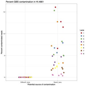
Considering the amount of sequencing coming out of the newer Illumina machines, we’ve started to combine GBS libraries with other samples. Due to how GBS libraries are made, when multiplexed with whole genome sequencing samples, there is an appreciable amount of contamination from GBS to WGS. That means you will find GBS reads in your WGS data. I’ve quantified that in the following figure, showing the percent of barcoded reads in WGS samples.

The left side is contamination from barcodes sequenced in different lanes (i.e. ones where they couldn’t contaminate). The right side is barcodes from GBS samples sharing the same lane (i.e. ones that could contaminate. The take home message is that between 1% to 15% of reads are GBS contamination. This is far above what we want to accept so they should be removed.

I’ve written a script to purge barcoded reads from samples. You give it the set of possible barcodes, both forward and reverse (All current barcodes listed here: GBS_2enzyme_barcodes). I’ve been conservative and been giving it all possible barcodes, but you could also trim it to only the barcodes that would be present in the lane. It looks for reads that start with the barcode (or any sequence 1bp away from the barcode to account for sequencing error) plus the cut site. If it finds a barcoded read, it removes both directions of reads. It outputs some stats at the end to STDERR. Note, this was written for 2-enzyme PstI-MspI GBS, although could be rewritten for other combinations.

An example of how you could apply this:

Make a bash script to run the perl script:

input=$1
perl ../purge_GBS_contamination.pl /home/gowens/bin/GBS_2enzyme_barcodes.txt ${input}_R1.fastq.gz ${input}_R2.fastq.gz ${input}.tmp;
gzip ${input}.tmp_R*.fastq

Run this bash script using gnu parallel

ls | grep .gz$ | grep R1 | sed s/_R1.fastq.gz//g | parallel -j 10 bash .decontaminate.sh 2>> decontamination_log.txt


Filtering TEs from SNP sets

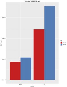
I’ve often wondered if the TEs in the sunflower genome were producing erroneous SNPs. I have unintentionally produced a little test of this. When calling SNPs for 343 H. annuus WGS samples I set FreeBayes to only call variants in non-TE parts of the genome (as per our TE annotations). Unfortunately, I coded those regions wrong, and actually called about 50% TE regions and 50% non-TE regions. That first set was practically unfiltered, although only SNPs were kept. I then filtered that set to select high quality SNPs (“AB > 0.4 & AB < 0.6 & MQM > 40 & AC > 2 & AN > 343 genotypes filtered with: DP > 2”). For each of these, I then went back in and removed SNPs from TE regions, and I’ve plotted totals below:

There are a few things we can take from this:

  • There are fewer SNPs in TE regions than non-TE regions. Even though the original set was about 50/50, about 70% of SNPs were from the non-TE regions.
  • For high quality SNPs, this bias is increased. 80% of the filtered SNPs were from non-TE regions.

Overall, I think this suggests that the plan to only call SNPs in non-TE regions is supported by the data. This has the advantage of reducing the genome from 3.5GB to 1.1GB, saving a bunch of computing time.

Comparing aligners

When analyzing genomic data, we first need to align to the genome. There are a lot of possible choices in this, including BWA (medium choice), stampy (very accurate) and bowtie2 (very fast). Recently a new aligner came out, NextGenMap. It claims to be both faster and deal with divergent read data better than other methods. Continue reading

Second barcode set

There is now a second set of barcoded adapters that allows higher multiplexing. They also appear to address the quality issues which have been observed in the second read of GBS runs.

This blog post has 1) Info on how to use the barcodes and where they are and 2) some data that might convince you to use them.

Usage

These add a second barcode to the start of the second read before the MSP RE site. The first bases of the second read contain the barcode, just like with the first read. Marco T. designed and ordered these and the info needed to order them is here: https://docs.google.com/spreadsheets/d/1ZXuHKfaR1BYPBX6g0p9GdZHp_21A3z_9pPt_aW0amwM/edit?usp=sharing

I’ve labeled them MTC1-12 and the barcode sequences are as follows.

MTC1 AACT
MTC2 CCAG
MTC3 TTGA
MTC4 GGTCA
MTC5 AACAT
MTC6 CCACG
MTC7 CTTGTA
MTC8 TCGTAT
MTC9 GGACGT
MTC10 AACAGAT
MTC11 CTTGTTA
MTC12 TCGTAAT

They are used in place of the common adapter in the standard protocol (1ul/sample). One possible use, and simplest to use as an example, would be to use these to run 12 plates in a lane. In this case you would make a master mix for the ligation of each plate which contains a different MTC adapter.

Where are they? In the -20 at the back left corner of the bay on the bottom shelf in a box that has a pink lab tape label that says something to the extent of “barcodes + barcoded adapters 1-12”. This contains the working concentration for each of the MTC adapters. Beside that is a box containing the unannealed and as ordered oligos and the annealed stock. The information regarding what I did and what is in the box is written there. The stock needs an additional 1/20 dilution to get to the working concentration

How it looks

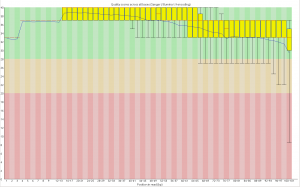
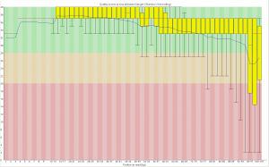
First, the quality of the second read is just about as nice as the first read. Using fastqc to look at 4million reads of some random run:

Read one:
R1_fastqc_quality

Read two:
R2_fastqc_report

Now, for the slightly more idiosyncratic part: read counts. In short I dont see any obvious issue with any of these barcodes. I did 5 sets of 5 plates/lane. For all the plates I used the 97-192 bacodes for the Pst side. Then each plate got a differnt MTC barcode for the MSP side. Following the PCR I pooled all of the samples from the plate and quantified. Each plate had a different number of samples which I took into account during the pooling step. Here is the read counts from a randomly selected 4 million reads corrected to number of samples in that plate. Like I said it is a little idiosyncratic but the take home is that they are about as even as you might expect given usual in accuracies in the lab, my hands, and the fact that this is a relatively small sample.

Lane 1
MTC5	14464
MTC1	13518
MTC7	14463
MTC9	13448
MTC3	14232

Lane 2	
MTC10	30395
MTC6	11267
MTC2	8263
MTC4	19295
MTC8	14766

Lane 3	
MTC5	16631
MTC7	17315
MTC11	11623
MTC9	16256
MTC3	13831

Lane 4		
MTC10	11302
MTC6	12120
MTC4	10326
MTC12	18959
MTC8	12832
	
Lane 5
MTC1	13151
MTC6	13490
MTC2	12851
MTC11	12460
MTC12	17296

Splits tree and iupac coding

I’ve been running splitstree to see the relationships between samples of H. bolanderi. I have coded my data using IUPAC so hets are a different symbol (Y, W, etc). The other way to code heterozygous sites into fasta is just pick one allele randomly.

By default, splitstree ignores all ambiguous sites, so if you use IUPAC coding, it will ignore all those sites. I switched it from ignoring, to using an average for all possible alleles. This made my tree much messier and had a weird smattering of samples pulled toward the outgroup. I’ve figured out that it has to do with the amount of missing data. Since Ns are ambiguous, when you average N it just sort of homogenizes the distances between samples. Thus, it can pull your samples into weird positions if they have different amounts of missing data.

My thoughts are that you should just ignore ambiguous data if you have enough sites to resolve your samples without them.

Sample Information Table

There is a constant problem of record keeping in the lab, and it is the most annoying in regards to sequence data. We have lots of data but finding out exactly what plants the data came from is difficult. So, I’m taking the old sample information table Seb made years ago and making it mandatory.

You must fill out this form before you get access to your sequence data. There will be one row per sample, meaning that for a GBS library you will have 96 or 192 rows.

Sample information table

Need cM positions?

Hello,

For a lot of work, it is helpful to know the cM position of your snps. Here is a script that takes the linkage map produced by Chris, your snp table in Hapmap format, and adds a column giving you a cM position for each site. It interpolates between known positions, so individual positions the accuracy of the position is overstated, but it’s good for plotting.

https://github.com/owensgl/reformat/blob/master/hmp2cmpositions.pl

usage:

perl hmp2cmpositions.pl /moonriseNFS/HA412/pseudomolecules/lg.ALL.bronze14.path.txt yoursnptable.hmp > yoursnptable.withcm.hmp


SmartGit GUI Tool

NOTE: This is an old draft post from Thuy (last updated 17 Dec 2012). I’m publishing it because it seems useful and mainly complete. –Brook

What is Git?

Git is a distributed source control version system.  It allows multiple people to work on the same code simultaneously by keeping track of changes made to files.  It visualizes differences between file versions and merges changes from different authors.  It also makes snapshots of file versions, so that you can go back to any version later.  Because git is distributed, you store a copy of the code repository and its change history on your own local machine.  When you are ready, you can sync your files to a remote repository server, such as BitBucket or GitHub.  Syncing to the remote server will share the updated code with all the other users, and they can merge the changes into their own copies if they wish.  Whether or not you use a remote repository server, git will always store your entire repository change history on your local machine.

Continue reading

Phred score detector

When using old sequence data you have to know what phred score system it is using. Almost all new data is going to use Phred33, but the old stuff could also be Phred64. There are scripts on this website that have ways of automatically detecting it http://wiki.bits.vib.be/index.php/Identify_the_Phred_scale_of_quality_scores_used_in_fastQ

I took the perl script from this website and parred down the output so that it works in pipelines. It outputs either “phred33” or “phred64”

fastq_detect_minimal.pl

An example pipeline in bash is:

coding=”$(perl $bin/fastq_detect_minimal.pl ${name}_1.fq)”

java -jar trimmmomatic-0.32.jar -$coding sample1.fq ….etc

NOTE: Phred64 should only go up to 104. There are some RNA seq samples (and probably others) that go up to 105. The original script output an error, while my version just says phred64. I hope that running it through phred conversion in trimmomatic fixes the issue but I am not sure.

2 enzyme GBS UNEAK trickery

Want to run UNEAK on a bunch of samples that you sequenced using 2 enzyme GBS? You came to the right place!

This takes R1.fastq.gz and R2.fastq.gz files and makes a single file containing both reads with the appropriate barcodes put on read 2 and the CGG RE site changed to the Pst sequence. This lets you use all of your data in UNEAK… well at least the first 64 bases of all your data!

This also deals with the fact that we get data that is from one lane but split into many files. See example LaneInfo file*. You will also need an appropriately formatted UNEAK key file.

*Only list READ1 in this file. It will only work if your files are named /dir/dir/dir/ABC_R1.fastq.gz and /dir/dir/dir/ABC_R2.fastq.gz.

so the file would read:
/dir/dir/dir/ ABC_R1.fastq C5CDUACXX 3

This is also made to work with .gz fastq files.

usage:
greg@computer$ perl bin/MultiLane_UneakTricker.pl design/UNEAK_KEY_FILE design/LaneInfo.txt /home/greg/project/UNEAK/Illumina

You must have the GBS_Fastq_BarcodeAdder_2Enzyme.pl* in the same bin folder. You also need to make a “tmp” folder.

LaneInfo
MultiLane_UneakTricker_v2
GBS_Fastq_BarcodeAdder_2Enzyme_v2

protip: UNEAK will be fooled by soft links so you can use them instead of copying your data.

Percent reads aligned collector

When you publish next gen sequencing data you have to include the percent reads aligned. The number is easy to get but when you have 200+ samples it’s a pain to collate them together. This script takes a directory with bam files, uses samtools flagstat to get percent reads aligned and then does a little rejiggering of format to put it in a nice list. To run it, enter the directory with the bams and type ‘bash ./percent_counter.bash’

percent_counter.bash NOTE: The script is gzipped.

Tassel 5

Tassel 5.0 is out and include many GBS functions. Although it is GWAS oriented it could still do a lot of preprocessing for other purposes:

  • Bit level encoding of nucleotides so genetic distance and linkage disequilibrium estimates can be made very quickly (20-50X speed increases).
  • Extensive use the HDF5 file format, which has been developed as a robust element of many climate modelers for matrix style data
  • Tools for extracting and calling SNPs from extensive Genotyping-by-Sequencing data (tested for 60,000 samples by over 2.5 million SNPs and 96 million sequence alleles).
  • Projection and imputation procedures that are optimized for the large families in crops.  Some of these optimizations permit memory and computational improvements of >100,000 fold.
  • Mixed models based on DNA relationships have come to dominate GWP (Meuwissen et al 2001) and GWAS (Yu et al 2006), yet these models can be slow to solve.  TASSEL has been a test bed and implements some of the most best optimizations, such as EMMA (Kang at al 2008), plus approaches optimize variance components once P3D (Zhang et al 2010) and EMMAX (Kang et al 2010).  Compression algorithms are also available (Zhang et al 2010).  When used correctly, these optimizations make powerful GWAS computationally possible.
  • The code is being continually optimized for larger numbers of cores and clusters.  For example, we generally run imputation on 64-core machines.  And while Java provides some excellent is interoperability between systems, its code is about 2-fold slower than optimized C libraries, and 10-fold slower than GPU processing for some problems.  TASSEL5 is building out connection layers directly to native code, when these efficiencies are need.

Non-Batch Submissions to the SRA

Since many of you have smaller amounts of data (a handful of samples/runs per experiment), I wanted to provide some info on submitting that data to the SRA without the help of their staff. The SRA has recently re-vamped their submission process, and it is much easier/simpler than before.

It’s important that everyone submit their own data. The SRA provides a free off-site backup, and we have already replaced corrupted files on our computers with clean copies obtained from the SRA. The time you spend doing this will ensure that you always have a clean copy of your raw data.

Here is a brief overview of the submission process, as well as the info you’ll need.

As well as the NCBI’s “quick start guide”.

Here are the pages for submitting BioProjects and BioSamples:

The process now is fairly straightforward and well-documented by the SRA. If anyone has trouble, you can ask others in the lab that have submitted their own data in the last year or so. I believe Dan Bock is one of them.

Here are some of the lab’s existing bioprojects. These can give you an idea of what kind of info to include in the abstract/project description, etc.:
http://www.ncbi.nlm.nih.gov/bioproject/PRJNA64989
http://www.ncbi.nlm.nih.gov/bioproject/PRJNA194568
http://www.ncbi.nlm.nih.gov/bioproject/PRJNA194569
http://www.ncbi.nlm.nih.gov/bioproject/PRJNA194570
http://www.ncbi.nlm.nih.gov/bioproject/PRJNA194446
http://www.ncbi.nlm.nih.gov/bioproject/PRJNA194445

The limits of GBS sample size

Image

I’ve been doing work on a stickleback GBS dataset and we’re trying to figure out how many samples we can cram into a single lane of illumina. I did some analyses which people may find useful. It’s unclear how applicable the recommendations are for sunflower which seems to have more problems than fish.

Take home message, with 25% less data you lose around 15% of the genotype calls, but up to 50% of the SNPs if you use a stringent coverage filter, due to how the lost data is distributed among loci and individuals.

Mounting the Moonrise NFS

Edit: As of February 2015, all our servers are running CentOS 7. The original instructions below are for Debian/Ubuntu linux, but here is a better set of generalized instructions for CentOS: https://www.howtoforge.com/nfs-server-and-client-on-centos-7

If you are mounting on an Ubuntu/Debian system, you can still use the instructions below. If you are mounting on a Red Hat derivative (Fedora, RHEL, CentOS, ScientificLinux, etc.), the link above should work.


I just had to re-learn how to do this today, so I thought it would be a good idea to write it up.

If any of you would like to mount the NFS on a computer (Unix, and static IPs only. This means no wireless!) in the building, you can do so at your convenience using this guide.

First, install nfs-common with your package manager (ubuntu: apt-get install nfs-common)

Next, create a folder for the mount to bind to on your computer, and make sure the permissions are set to 777:

user@mycomputer: mkdir -p /nameofyourNFSfolder
user@mycomputer: chmod 777 /nameofyourNFSfolder

I think the whole tree needs the same permissions, so what I’ve done for all our machines (and what seems easiest) is to make a folder in the root directory, so that you don’t have to worry about the permissions in parent folders.

Next, the /etc/hosts.allowed and /etc/exports files on moonrise need to be modified. Chris, Frances, and I all have the necessary permissions to do this. Just ask one of us and we can do it.

root@mooonrise: nano /etc/exports

Add the following to the line beginning with /data/raid5part1
137.82.4.XXX(rw,sync) (with XXX standing in for the static IP of your machine)

You could also do this with machines in other buildings/off-campus as long as their IPs are static.

root@moonrise: nano /etc/hosts.allow

Your IP has to be added to the end of each line in this file.

Now reload the /etc/exports file on moonrise (a full NFS restart is not required, and will unmount it on other machines! don’t do that unless you know for sure that no one is using the NFS on any of our computers!)

root@moonrise: exportfs -a

Finally, mount the NFS on your machine:

user@mycomputer: sudo mount -v -o nolock -t nfs moonrise.zoology.ubc.ca:/data/raid5part1 /nameofyourNFSfolder

There are various options you can use with the mount command, but the above should work for just about anyone.

If you want it to auto-mount each time you boot your computer, you can add the following lines to your /etc/fstab file:
#moonriseNFS
137.82.4.123:/data/raid5part1 /nameofyourNFSfolder nfs auto 0 0

That’s it!

SNP calling with GATK warning

I’ve come to the realization that I’ve been making a mistake in my SNP calling using GATK. I’ve been filtering for site quality not for individual genotype quality. This is a critical difference and leads to some dubious SNPs being called.

It works like this. For each position in the genome, GATK will use all the data together to call whether an alternate allele exists. This is represented by the phred scaled QUAL score. A high QUAL score means that the alternate allele exists in in your dataset. This number is often very high if you’re analyzing a whole plate of GBS because it takes into account all the data from all the individuals. I’ve been filtering based on this number.

There is also a MQ score, which is the mapping quality for all the reads at that site.

For each individual, if there are any reads at that site GATK will output a genotype call (i.e. 0/0, 0/1, 1/1). It also outputs the number of reads supporting each allele, the QT score (which is the phred scaled probability of that the genotype call being correct) and the likelihoods of each possible genotype. When you use select variants in GATK, it filters sites but not genotypes (so you can have a site that is good, but individual genotype calls at that site that are bad).

If you use vcf-to-tab to convert your vcf to tab separated it will accept every genotype call. This means that for some individuals you will have 1 read supporting the reference and it will be called as 0/0. The QT score will be 3, which is incredibly low, but vcf-to-tab ignores that information and calls it. Therefore a proportion of your SNPs are highly questionable. This likely contributes to the heterozygote loss seen in GBS data.

Sam and Chris wrote a script that converts a vcf file to tab but also makes sure that the quality (QUAL, QT, MQ, and depth) is good. I’ll post it if they’re OK with it be up.

Edit: Here are the scripts. They are identical except one outputs in IUPAC format (AT=W, AC=M, etc) and the other outputs in the standard double nucleotide format (AA, AT, etc).vcf2vertical_dep_GATK-UG vcf2vertical_dep_GATK

Also note that sometimes GATK will output a genotype call that looks like:

./.:.:3

While normally they should look like:

./. or 0/0:17,0:18:45:0,45,353

This is saying that there are three reads at this position, but the quality is so bad that GATK is not calling the genotype. If you have these, the scripts will throw an error but will correctly output an NN for that genotype. So if you get a normal output and many errors, it’s probably OK.