BayEnv

Apparently BayEnv is the way to do differentiation scans. Here I offer some scripts and advice to help the you use Bayenv.

Install, no problem get it here: http://gcbias.org/bayenv/ Unzip.

I have to say the documentation is not very good.

There is 2 things you will probably want to use BayEnv for:
1) Environmental correlations
2) XtX population differentiation
I will just be showing XtX here. Both need a covariance matrix. This is not the “matrix.out” file you get from the matrix estimation step.
. But first the SNP table.

Here is a script Greg O made to make a “SNPSFILE”* for bayenv from our standard SNP table format: SNPtable2bayenv I’ve made a small modification so that it excludes any non-bi-allelic site and to also print out a loci info file.
Use it like this:

perl SNPtable2bayenv.pl SNPfile POPfile SampleFile

This will make three files with “SampleFile” appended to the start of the name.
*not actually a SNP file at all, it is an allele count file.

Input SNPfile (all spaces are tabs):

CHROM POS S1 S2 S3 S4 S5
chr1 378627 AA TT NN TT AA
chr2 378661 AA AG NN GG AA
chr3 378746 GG AA NN AA GG
chr4 383246 NN GG NN GG TT
chr5 397421 CC GG NN GG CC
chr6 397424 GG AA NN AA GG
chr7 409691 NN CC NN NN GG
chr8 547653 AA GG NN GG AA
chr9 608412 AA GG NN NN AA
chr10 756412 GG CC NN CC GG
chr11 1065242 NN TT NN NN CC
chr12 1107672 NN TT NN TT NN

POPfile (all spaces are tabs):

S1 p1
S2 p1
S3 p2
S4 p2
...

Now estimate the covarience matrix:

./bayenv2 -i SampleFile.bayenv.txt -p 2 -k 100000 -r21345 > matrix.out

Now this is “matrix.out” file is not what you actually want. You have to use it to make a new file that contains a single covariance matrix. You could use “tail -n3 matrix.out | head -n2 > CovMatrix” or just cut it out yourself. Currently I am just using the last (and hopefully converged) values.
My CovMatrix.txt looks like this (again single tabs between):

3.009807e-05 -1.147699e-07   
-1.147699e-07 2.981001e-05

You will also need a environment file. I am not doing the association analysis so am just using some fake data. It is one column for each population and each row is the environmental values. Tab separated.
FakeEnv.txt

1 2

Now you can do the population differentiation test for each snp using a “SNPFILE”. I bet you think you are ready to go? Not so fast, you need a “SNPFILE” not a “SNPSFILE”. Not that either actually really have SNPs in them, just allele counts. Not that I am bitter. SNPFILE is just one site from the SNPSFILE. Here is a script that takes your “SNPSFILE” and runs the XtX program on each of the sites: RunBayenvXtX

perl RunBayenvXtX.pl SampleFile.bayenv.txt SampleFile.LocInfo.txt CovMatrix.txt FakeEnv.txt 2 1 

Where 2 is the number of populations and 1 is the number of environmental variables.
This will produce a file that has the site, allelecountfile name and the XtX value.

Approximate Bayesian Computations

In many cases it may be more straightforward (and informative) to test specific models using our data. An interesting approach for inferring population parameters and/or model testing is approximate Bayesian computations (ABC). There are several available tools such as msBayes, DIYABC, PopABC abctools R package, ABCTools.

Although ABC is a powerful and useful approach it has some caveats, e.g. choice of summary statistics, number and complexity of the models tested, amount of data and more. For realistic expectations and simple models ABC could really add some interesting insights to popgen studies.

Paired End for Stacks and UNEAK

Both stacks and uneak are made for single end reads. If you have paired end data here is a little cheat that puts “fake” barcodes onto the mate pairs and prints them all out to one file. It also adds the corresponding fake quality scores.

perl GBS_fastq_RE-multiplexer_v1.pl BarcodeFile R1.fastq R2.fastq Re-barcoded.fastq

BarcodeFile should look like (same as for my demultiplexing script) spaces must be tabs:
sample1 ATCAC
sample2 TGCT

# note this could also look like this:
ATCAG ATCAG
TGCT TGCT

As it does not actually use the names (it just looks at the second column).

Here it is:
GBS_fastq_RE-multiplexer_v1

actual UNEAK

Some of you may have heard me ramble about my little in house Uneak-like SNP calling approach. I am being converted to using the actual UNEAK pipeline. Why? reason #1 is good god is it fast! I processed 6 lanes raw fastq to snp table in ~1 hour. #2 I am still working on – this will be a comparison of SNP calls between a few methods but I have a good feeling about UNEAK right now.

Here is the UNEAK documentation: http://www.maizegenetics.net/images/stories/bioinformatics/TASSEL/uneak_pipleline_documentation.pdf

It is a little touchy to get it working so I thought I would post so you can avoid these problems.

First install tassel3 (not tassel 4) you will need java 6 or younger to support it: http://www.maizegenetics.net/index.php?option=com_content&task=view&id=89&Itemid=119

To be a hacker turn up the max RAM allocation. Edit run_pipeline.pl to change the line “my $java_mem_max_default = “–Xmx1536m”;” to read something like “my $java_mem_max_default = “–Xmx4g”;” (That is 4g for 4G of RAM).

Go to where you want to do the analysis. This should probably be a new and empty directory. Uneak starts by crawling around looking for fastq files so if the directory has some files you don’t want it using it is going to be unhappy.
Make the directory structure:

../bin/run_pipeline.pl -fork1 -UCreatWorkingDirPlugin -w /home/greg/project/UNEAK/ -endPlugin -runfork1 

Move your raw (read: not demultiplexed) fastq or qseq to /Illumina/. If you are using fastq files the names need to look like this: 74PEWAAXX_2_fastq.txt NOT like this:74PAWAAXX_2.fastq and probably not a bunch of other ways. It has to be flow cell name underscore lane number understore fastq dot txt. You might find others work but I know this does (and others don’t).
Make a key file. This is as described in the documentation. It does not have to be complete (every location on the plate) or sorted. Put it in /key/

Flowcell        Lane    Barcode Sample  PlateName       Row     Column
74PEWAAXX       1       CTCGCAAG        425218  MyPlate7        A       1
74PEWAAXX       1       TCCGAAG 425230  MyPlate7        B       1
74PEWAAXX       1       TTCAGA  425242  MyPlate7        C       1
74PEWAAXX       1       ATGATG  425254  MyPlate7        D       1
...

Run it. Barely enough time for coffee.

../bin/tassel3.0_standalone/run_pipeline.pl -fork1 -UFastqToTagCountPlugin -w /home/greg/project/UNEAK/ -e PstI -endPlugin -runfork1
# -c how many times you need to see a tag for it to be included in the network analysis
../bin/tassel3.0_standalone/run_pipeline.pl -fork1 -UMergeTaxaTagCountPlugin -w /home/greg/project/UNEAK/ -c 5 -endPlugin -runfork1
# -e is the "error tolerance rate" although it is not clear to me how this stat is generated
../bin/tassel3.0_standalone/run_pipeline.pl -fork1 -UTagCountToTagPairPlugin -w /home/greg/project/UNEAK/ -e 0.03 -endPlugin -runfork1
../bin/tassel3.0_standalone/run_pipeline.pl -fork1 -UTagPairToTBTPlugin -w /home/greg/project/UNEAK/ -endPlugin -runfork1
../bin/tassel3.0_standalone/run_pipeline.pl -fork1 -UTBTToMapInfoPlugin -w /home/greg/project/UNEAK/ -endPlugin -runfork1
#choose minor and max allele freq
../bin/tassel3.0_standalone/run_pipeline.pl -fork1 -UMapInfoToHapMapPlugin -w /home/greg/project/UNEAK/ -mnMAF 0.01 -mxMAF 0.5 -mnC 0 -mxC 1 -endPlugin -runfork1

Some bioinformatics tools

New tools for analyzing NGS are coming out occasionally. Usually we tend to stick to the same tools just because they work. Well, you may find new tools faster or more accurate for your purposes. Here is a list of tools (and links) which could be used for different purposes (not only RNA-Seq). I could recommend FastQC, FastX, and trimmomatic for cleaning any raw data, and sabre is a nice tool to clean GBS.
FLASH works well for merging reads (there are more tools though) and this seems to be an interesting pre-processing approach. As for sequence aligners, except for bowtie and bwa you may find subread to be fast due to it’s different approach and additional complementary tools for splice alignments, feature counting and SNP calling. Another interesting aligner is stampy which enable to align reads to a diverged reference genome but need some pre- and post- processing to get fast results, otherwise it takes forever.

Of course, there are also some more ‘traditional’ tools for aligning bigger sequences such as MUMer (nucmer, promer) and AMOS. Although these tools are powerful they need some extra pre/post processing which is not always appreciated.

fastSTRUCTURE is fast.

fastSTRUCTURE is 2 orders of magnitude faster than structure. For everyone who has waited for structure to run this should make you happy.
Preprint of the manuscript describing it here: http://biorxiv.org/content/early/2013/12/02/001073

UPDATE comparison: Structure_v_FastStructure Structure (top) 8 days and counting FastStructure (below) 15 minutes. You can see the are nearly identical. I would expect them to be within the amount of variation you normally see on structure runs. Structure is only on K=4 (with 50,000 burnin and 100,000 reps and 5 reps of each K) where FastStructure took just under 15 minutes to go K of 1 to 10. Note: these are sorted by Q values not by individuals so, although I think it is highly unlikely, they may be discordant on an individual scale.

UPDATE on speed: ~400 individuals by ~4000 SNPs K=1 to K=10 in just under 15 minutes.

UPDATE on usage: Your structure input file must be labeled .str but in when you call the program leave the .str off. If you don’t adds it itself and will look for MySamples.str.str

It has a few dependencies which can make the installation a little intimidating. I found installing them was relatively easy and I downloaded everything, installed and tested it all in less than one hour.

The site to get fastSTRUCTURE:
http://rajanil.github.io/fastStructure/

You can follow along there, the instructions are pretty good. This is just what I did with a few notes.

At the top you can follow links to the dependencies.

Scipy + Cython

#Scipy
sudo apt-get install python-scipy python-sympy
#Cython
download + scp
tar -zxvf Cython-0.20.tar.gz
cd Cython-0.20/
make
sudo python setup.py install

Numpy

#probably the easiest way:
sudo apt-get install python-numpy python-nose

#what I did before I figured out above:
download + scp
tar -zxvf numpy-1.8.0.tar.gz
cd numpy-1.8.0
python setup.py build --fcompiler=gnu
#also installed "nose" similarly it is at least needed to run the test
#test
python -c 'import numpy; numpy.test()'

On to fastSTRUCTURE

wget --no-check-certificate https://github.com/rajanil/fastStructure/archive/master.tar.gz
#then
#check where GSL is
ls /usr/local/lib
# You should see a bunch of stuff starting with libgsl
# You can look in your LD_LIBRARY_PATH before adding that path
echo $LD_LIBRARY_PATH
# add it
export LD_LIBRARY_PATH=$LD_LIBRARY_PATH:/usr/local/lib
# check it worked
echo $LD_LIBRARY_PATH #mine only has ":/usr/local/lib" in it
#decompress the package
tar -zxvf master.tar.gz
cd fastStructure-master/vars/
python setup.py build_ext --inplace
cd ..
python setup.py build_ext --inplace
#test
python structure.py -K 3 --input=test/testdata --output=testoutput_simple --full --seed=100

GATK on sciborg

A few notes on GATK.
1. GATK requires a younger version of Java than what is on the cluster currently.
> java -jar ./bin/GenomeAnalysisTK-2.8-1-g932cd3a/GenomeAnalysisTK.jar --help                                                                                    Exception in thread "main" java.lang.UnsupportedClassVersionError: org/broadinstitute/sting/gatk/CommandLineGATK : Unsupported major.minor version 51.0
Get the linux 64 bit version here:
http://java.com/en/download/
move it to sciborg:
> scp ../Downloads/jdk-7u45-linux-x64.tar.gz user@zoology.ubc.ca:cluster/bin/
#ssh  to the cluster extract it:
> tar -zxvf jdk-7u45-linux-x64.tar.gz
#Add it to your path file or use it like so:
> ./bin/jdk1.7.0_45/bin/java -jar ./bin/GenomeAnalysisTK-2.8-1-g932cd3a/GenomeAnalysisTK.jar --help
2. You must have a reference with a relatively small number of contigs/scaffolds
Kay identified and addressed this problem and wrote this script: CombineScaffoldForGATK. I’ve modified it very slightly.
perl CombineScaffoldForGATK.pl GenomeWithManyScaffolds.fa tmp.fa
WARNING: this can print empty lines. The script could be modified to address this but I don’t want to break it. Instead you can fix it with a sed one liner:
sed '/^$/d' tmp.fa > GenomeWith1000Scaffolds.fa
3. You must also prepare the “fasta file”
You also have to index it for BWA with bwa index but GATK needs more, see: http://gatkforums.broadinstitute.org/discussion/1601/how-can-i-prepare-a-fasta-file-to-use-as-reference
In short (in the same dir as your genome):
>java -jar ../bin/picard-tools-1.105/CreateSequenceDictionary.jar R= Nov22k22.split.pheudoScf.fa O= Nov22k22.split.pheudoScf.dict
>samtools faidx Nov22k22.split.pheudoScf.fa

Where does all the GBS data go? Pt. 2

An analysis aimed at addressing some questions generated following discussion of a previous post on GBS

Number of fragments produced from a ‘digital digestion’ of the Nov22k22 Sunflower assembly:

Clai: 337,793
EcoRI: 449,770
SacI: 242,163
EcoT22I: 528,709
PstI: 129,993
SalI: 1,210,000
HpaII/MspI: 2,755,916

Here is the size distribution of those fragments (omitting fragments of >5000bp):
All the enzymes
With Msp removed for clarity

Take home message: PstI produces fewer fragments of an appropriate size than other enzymes. It looks like the correlation between total number of fragments and number that are the correct size is probably pretty high.

Now for a double digestion. Pst and Msp fragment sizes and again omitting fragments >5000bp. This looks good. In total fragment numbers (also omitting >5000bp fragments):

Pst+Msp total fragments: 187271
Pst+Msp 500<>300bp: 28930
Pst alone total: 79049
Pst alone 500<>300bp:6815

Take home: Two enzyme digestion could work really well. It may yield more than 4 times more usable fragments. I do think we could aim to get even more sites. Maybe some other RE combination could get us to the 100,000 range. With a couple of million reads per sample this could still yield (in an ideal world) 10x at each site. Send me more enzymes sequences and I can do more of the same.

Edited for clarity and changed the post name

Where does all the GBS data go?

Why do we get seemingly few SNPs with GBS data?

Methods: Used bash to count the occurrences of tags. Check your data and let me know what you find:

cat Demutliplexed.fastq | sed -n '2~4p' | cut -c4-70 | sort | uniq -c | grep -v N | sed 's/\s\s*/ /g' > TagCounts

Terminology: I have tried to use tags to refer to a particular sequence and reads as occurrences of those sequences. So a tag may be found 20 times in a sample (20 reads of that sequence).

Findings: Tag repeat distribution

Probably the key thing and a big issue with GBS is the number of times each tag gets sequence. Most sites get sequenced once but most tags get sequence many many times. It is hard to see but here are histograms of the number of times each tags occur for a random sample (my pet11): All tags histogram (note how long the x axis is), 50 tags or less Histogram. Most tags occur once – that is the spike at 1. The tail is long and important. Although only one tag occurs 1088 times it ‘takes up’ 1088 reads.

How does this add up?

In this sample there are 3,453,575 reads. These reads correspond to 376,036 different tag sequences. This would mean (ideally) ~10x depth of each of the tags. This is not the case. There are a mere 718 tags which occur 1000 or more times but they account for 1394905 reads. That is 40% of the reads going to just over 700 (potential) sites. I’ve not looked summarized more samples using the same method but I am sure it would to yield the same result.

Here is an example: Random Deep Tag. Looking at this you can see that the problem is worse than just re-sequencing the same tag many times but you introduce a large number of tags that are sequencing and/or PCR errors that occur once or twice (I cut off many more occurances here).

Conclusion: Poor/incomplete digestion -> few sites get adapters -> they get amplified like crazy and then sequenced.

Update 1:

Of the > 3.4Million tags that are in the set of 18 samples I am playing with only 8123 are in 10 or more of the samples.

For those sites with >10 scored the number of times a tag is sequenced is correlated between samples. The same tags are being sequenced repeatedly in the different samples.

Update 2:

As requested the ‘connectivity’ between tags. This is the number of 1bp miss matches each tag has. To be included in this analysis a tag must occur at least 5 times in 3 individuals. Here is the figure. So most tags have zero matches a smaller number have one and so on. This actually looks pretty good – at least how I am thinking about it now. This could mean that the filtering criteria works. If errors were still being included I would expect tags with one match (the actual sequence) to occur more than ones with zero.

Quick phylogenetic trees colored by trait in R

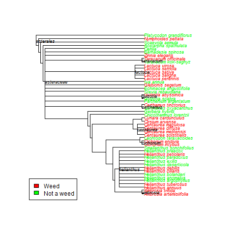
Basically, here is some easy code to search publicly available databases to determine a trait value for a species (in this case whether or not the species was recorded as invasive in any of 5 global invasive species databases), then make a quick tree based on published phylogenies using Phylomatic (http://phylodiversity.net/phylomatic/), then color code the tree based on the trait value.

Subset of species from Asteraceae and whether they have been reported as invasive ('weedy') in any of 5 global invasive species databases.

Subset of species from Asteraceae and whether they have been reported as invasive (‘weedy’) in any of 5 global invasive species databases.

Continue reading

Turning STACKS output into IMa2 input files

This script extract sequence haplotypes from the “alleles.tsv” files generated by STACKS and does some light filtering (you may want to add more). It’s very similar to the one I used for our 2013 Molecular Ecology paper, and still has some Great Sand Dunes-specific parameter names, but should work ok for other data sets. Oh, and I was using the “pstacks” reference-guided workflow in a slightly older version STACKS, in case that matters.

extract_haplotype_sequences_v4_annotated.r

example_alleles.tsv

Please let me know if you use this script and whether it needs tweaking.

Sequencing Data Organization Update

Image

I’ve created a skeleton directory structure and included a few example folders so that everyone can get a better idea of how our data will be organized on the new sever. These are not set in stone. A few people have commented on the blog, or in lab meeting, or to me in person, and I’ve taken all of your suggestions into account.

If you feel like the setup here isn’t optimal, please give some feedback. The better we do this now, the more smoothly things will run in the future!

Sequencing Data Curation Part 1

With our new data server (Moonrise) up and ready to store our sequences, it is time to start being more careful about where and when we move our most important data, and how we keep track of it. I’ve devised a system for storing our data for those of you who will be accessing it via the servers. Only Chris, Sariel, Frances and I will have write access to the directories where data is stored. If you would like your data stored, you will have to fill out a form which I’ve created which will give us all the information we need to store it in its right place. Here is the form.

This is inserting a little bureaucracy into our system, and it’s going to be a pain, but in the long run it will make things much easier. We currently have data which we had a very difficult time finding because the owner is no longer in the lab. With a system like the new one, that will not happen.

We will store our WGS, RNASeq, and GBS data in separate folders. This will make finding your data easier in most cases.

Here are the directory structures for the three types of data:

WGS -> Species -> Cultivar -> Library -> Experiment -> file_name_including_library_size_and_depth_coverage.fq METADATA.txt

RNASeq -> Experiment  (if unnecessary, the following directories can be omitted) -> Species -> Cultivar/Population -> Library -> file_name_including_library_size_and_depth_coverage.fq METADATA.txt

GBS is a little more complex, and we will separate things in two ways.
GBS -> Cut Site/Enzyme (data with different cut sites might be incompatible) -> Data type (population genetics, mapping data) -> From here on things diverge
Pop -> Group* -> files_with_descriptive_names.fq METADATA.txt
Map -> Experiment -> Species -> files_with_descriptive_names.fq METADATA.txt
*groups are based loosely on clades, and on how much data for each species we have (annuus_wild, annuus_cult, argophyllus, bolanderi_exilus, petiolaris_clade, hybrids, perennials, tuberosus_cult)

Generally, file names should include data not encoded in the directory structure, but important enough to be seen when perusing the data. Things like depth of coverage, library size, etc. seem appropriate for all three data types, but for types with which I’m not as familar (GBS), suggestions would be appreciated.

GBS, coverage and heterozygosity. Part 3

I’ve recalled the SNPs for my Helianthus exilis population genetics for a third time. This time I’m using GATK. This is aligned using BWA to the Nov22k22 reference.

This is two plates of GBS (96-plex each) plus 34 H. annuus samples from G. Baute (also 96-plex GBS). Three exilis samples were removed because they had little or no reads. Reads were trimmed for adapters and quality using trimmomatic (and the number of  reads kept after trimming are used here).

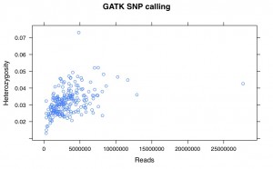
Exil.GATK.file.het


So, there is a relationship between number of reads and resulting heterozygosity. It makes some sense because you need a higher number of reads to call a heterozygote than a homozygote. It’s not as bad as what was happening when we were calling snps using the maximum likelihood script. Using a linear model, number of reads accounts for %16 of the variation in heterozygosity.

If you compare this to my previous posts, the heterozygosity is vastly lower for all samples. That is because I previously looked at variable sites with a certain amount of coverage, and here are all sites. So a majority of these sites are invariant.


SNP calling V – SNP and genotype calling

The next step in the pipeline after the alignments are conducted and adjusted is to call the SNPs and genotypes. There are many programs that will do this such as the ML script that many people in the Rieseberg lab use, freeBayes, mpileup and bcftools, as well as the GATK UnifiedGenotyper. To bench mark the alignment steps in these SNP calling blog posts I used mpileup and bcftools. For example:

Continue reading

SNP calling IV – Base quality score recalibration

The best practices protocol from Broad highly recommends base quality recalibration (http://gatkforums.broadinstitute.org/discussion/44/base-quality-score-recalibration-bqsr). Apparently, the base quality scores off the machine are not very accurate and can provide false confidence in the base calls and consequently influence SNP calling. This tool will adjust average quality scores and also adjust the scores depending on the machine cycle and sequence context (i.e. start versus end of read, type of dinucleotide repeat). After recalibration, the quality score is closer to its actual probability of mismatching the reference genome.

To run this you need a database of known SNPs so the tool can assess the error rate at other sites based on the actual sequence data. Unlike humans, which this tool was designed for, most species do not have comprehensive SNP databases. However, such a table can be created by identifying SNPs in a preliminary run without the base quality score recalibration. I included any SNP that had a Qual score of 20 in my SNP vcf file.

You can see below that it had a large effect on the number of SNPs that I called. With the BAQ filter off 263,360 SNPS overlapped between the methods. 14,591 were unique to the recalibrated alignments and 131,354 were unique to the alignments without base quality recalibration.

Continue reading

SNP calling III – The indel problem

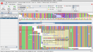
SNPs can often be falsely called around indels. In particular, if indels are near the start or end of a read the read is often incorrectly aligned. Here is an example of how things can go wrong from a spruce alignment. Below, at site 109 there is a TT insertion in the reads relative to the reference and there is no true SNP at this site. However, this individual was called as a het (C/T) because of the reads that end in the middle of the insertion. For these reads the penalty for a single mismatch to the reference is less than introducing a gap.

Screen Shot 2013-08-15 at 10.13.34 AM

Continue reading