We already have a GBS protocol on the lab blog, but since it contains three different variants (Kate’s, Brook’s and mine) it can be a bit messy to follow. Possibly because I am the only surviving member of the original trio of authors of the protocol, the approach I used seems to have become the standard in the lab, and Ivana was kind enough to distill it into a standalone protocol and add some additional notes and tips. Here it is!
Tag Archives: GBS
How to do effective SPRI beads cleaning
Reply
SPRI beads cleaning is one of the most repetitively used step during library preparations and probably the step where most of us lose a lot of precious DNAs.
Losing DNA scared me so much (because it can be observable) that I hesitated a lot before trying to use beads to concentrate genomic DNA, because usual rate of recovery are ~50%.

Hopefully with some practice and a lot of patience, it is possible to reach 90% recovery. How to lose as little DNA as possible? Here are some guidelines: Continue reading
How to do GBS libraries with “difficult” DNA samples
First of all, let’s be clear about it: Having good amount of high quality DNA should be a starting point for all projects. Recently, we had this conversation at lab meeting about the “one rule” to succeed in establishing a lab (quoting Loren): “Don’t try to save money on DNA extraction. Working with high quality DNA reduces cost at all downstream steps, even on bioinformatics”.
However, if you need to work with “historical” DNA samples from the lab (I genotyped old DNA plates at least 8 years old) or DNA from collaborator for which you have no control over the DNA quality and/or no more plant tissue to redo DNA extraction, here are some tips on how to get a maximum out of (almost) nothing.
I started the GBS protocol with 100ng of DNA, it works. However, if you want to save yourself a lot of time and the lab some money on repeating PCR, repeating samples, repeating a lot of qubit measurement, start with 200ng.
A) If some of your DNA samples are <8.5 ng/ul (100ng protocol):
Among the 1500 DNA samples I received from a collaborator, 134 did not meet the requirement (>8.5 ng/ul) to start the GBS. I thought about concentrating these DNA with different methods: 1) using beads: you need to be ready to loose 50% of the DNA; 2) speedvac: I did not find one (supposedly there is one in the Adams lab?) and I was concerned about over-concentrating TE in the same time as DNA.
Hopefully, if you look at the digestion step, a large volume of the digestion mix is water/tris. By removing this water, I was able to include in the protocol DNA with concentration >5.8ng/ul, recovering half of my problematic samples. Just be extra-careful when pipetting the 2.8 ul of “water-free” digestion master mix. I had good PCR amplification for these samples.
B) If you are desperate:
I used whole genome amplification (WGA) prior to starting the GBS protocol to increase the DNA concentration of “historical” DNA samples. You will probably recover most of your DNA samples if they are more than 1ng/ul.
However, DO NOT MIX genome amplified and plain genomic DNA on the same plate for sequencing, especially if you pool your library before doing PCR and qubiting. The WGA samples amplify much better and Sariel showed me libraries in which few WGA samples took a large part of the sequencing reads. It’s a recipe for disaster and high missing data.
My strategy was to qubit all the DNA plates and estimate the remaining volume. If the remaining DNA sample was less than 100ng, I did WGA but I moved these samples to specific WGA plates. It’s a bit more work because if your samples are already in plates, you will need to relocate all your samples. From my experience, it’s worth it.
Comparing aligners
When analyzing genomic data, we first need to align to the genome. There are a lot of possible choices in this, including BWA (medium choice), stampy (very accurate) and bowtie2 (very fast). Recently a new aligner came out, NextGenMap. It claims to be both faster and deal with divergent read data better than other methods. Continue reading
GBS barcodes 97-192
If you are using GBS barcodes 97 – 192, here is the sequence info (from Brook). This might be somewhere else on the blog, but I couldn’t find it! Also included, sequence info for barcodes 1 – 96.
Second barcode set
There is now a second set of barcoded adapters that allows higher multiplexing. They also appear to address the quality issues which have been observed in the second read of GBS runs.
This blog post has 1) Info on how to use the barcodes and where they are and 2) some data that might convince you to use them.
Usage
These add a second barcode to the start of the second read before the MSP RE site. The first bases of the second read contain the barcode, just like with the first read. Marco T. designed and ordered these and the info needed to order them is here: https://docs.google.com/spreadsheets/d/1ZXuHKfaR1BYPBX6g0p9GdZHp_21A3z_9pPt_aW0amwM/edit?usp=sharing
I’ve labeled them MTC1-12 and the barcode sequences are as follows.
MTC1 AACT
MTC2 CCAG
MTC3 TTGA
MTC4 GGTCA
MTC5 AACAT
MTC6 CCACG
MTC7 CTTGTA
MTC8 TCGTAT
MTC9 GGACGT
MTC10 AACAGAT
MTC11 CTTGTTA
MTC12 TCGTAAT
They are used in place of the common adapter in the standard protocol (1ul/sample). One possible use, and simplest to use as an example, would be to use these to run 12 plates in a lane. In this case you would make a master mix for the ligation of each plate which contains a different MTC adapter.
Where are they? In the -20 at the back left corner of the bay on the bottom shelf in a box that has a pink lab tape label that says something to the extent of “barcodes + barcoded adapters 1-12”. This contains the working concentration for each of the MTC adapters. Beside that is a box containing the unannealed and as ordered oligos and the annealed stock. The information regarding what I did and what is in the box is written there. The stock needs an additional 1/20 dilution to get to the working concentration
How it looks
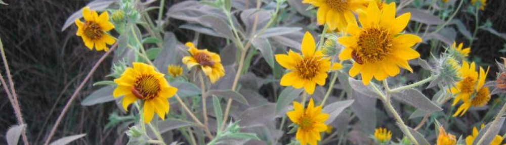
First, the quality of the second read is just about as nice as the first read. Using fastqc to look at 4million reads of some random run:
Read one:
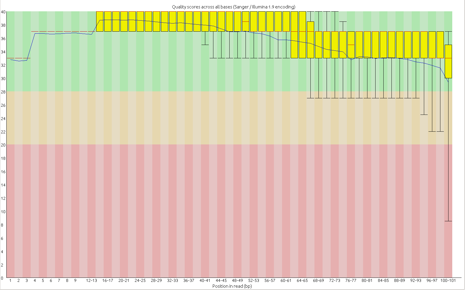
Read two:
Now, for the slightly more idiosyncratic part: read counts. In short I dont see any obvious issue with any of these barcodes. I did 5 sets of 5 plates/lane. For all the plates I used the 97-192 bacodes for the Pst side. Then each plate got a differnt MTC barcode for the MSP side. Following the PCR I pooled all of the samples from the plate and quantified. Each plate had a different number of samples which I took into account during the pooling step. Here is the read counts from a randomly selected 4 million reads corrected to number of samples in that plate. Like I said it is a little idiosyncratic but the take home is that they are about as even as you might expect given usual in accuracies in the lab, my hands, and the fact that this is a relatively small sample.
Lane 1
MTC5	14464
MTC1	13518
MTC7	14463
MTC9	13448
MTC3	14232

Lane 2
MTC10	30395
MTC6	11267
MTC2	8263
MTC4	19295
MTC8	14766

Lane 3
MTC5	16631
MTC7	17315
MTC11	11623
MTC9	16256
MTC3	13831

Lane 4
MTC10	11302
MTC6	12120
MTC4	10326
MTC12	18959
MTC8	12832

Lane 5
MTC1	13151
MTC6	13490
MTC2	12851
MTC11	12460
MTC12	17296
2 enzyme GBS UNEAK trickery
Want to run UNEAK on a bunch of samples that you sequenced using 2 enzyme GBS? You came to the right place!
This takes R1.fastq.gz and R2.fastq.gz files and makes a single file containing both reads with the appropriate barcodes put on read 2 and the CGG RE site changed to the Pst sequence. This lets you use all of your data in UNEAK… well at least the first 64 bases of all your data!
This also deals with the fact that we get data that is from one lane but split into many files. See example LaneInfo file*. You will also need an appropriately formatted UNEAK key file.
*Only list READ1 in this file. It will only work if your files are named /dir/dir/dir/ABC_R1.fastq.gz and /dir/dir/dir/ABC_R2.fastq.gz.
so the file would read:
/dir/dir/dir/ ABC_R1.fastq C5CDUACXX 3
This is also made to work with .gz fastq files.
usage:
greg@computer$ perl bin/MultiLane_UneakTricker.pl design/UNEAK_KEY_FILE design/LaneInfo.txt /home/greg/project/UNEAK/Illumina
You must have the GBS_Fastq_BarcodeAdder_2Enzyme.pl* in the same bin folder. You also need to make a “tmp” folder.
LaneInfo
MultiLane_UneakTricker_v2
GBS_Fastq_BarcodeAdder_2Enzyme_v2
protip: UNEAK will be fooled by soft links so you can use them instead of copying your data.
PstI-MspI GBS protocol
The “protocol” that we have been using is available here as a Google doc. I use quotes there because, as you will see, there is no single protocol used by the lab to date. Without analyzed sequence data yet to compare the described protocols, the best advice I can give to you is to pick a sensible pipeline for your needs, taking into consideration the time/effort/desired output that works for you, and apply that pipeline consistently to all samples for the same project. All sets of methods described have resulted in libraries that pass QC and generate a sufficient reads during sequencing. Good luck!
Tassel 5
Tassel 5.0 is out and include many GBS functions. Although it is GWAS oriented it could still do a lot of preprocessing for other purposes:
- Bit level encoding of nucleotides so genetic distance and linkage disequilibrium estimates can be made very quickly (20-50X speed increases).
- Extensive use the HDF5 file format, which has been developed as a robust element of many climate modelers for matrix style data
- Tools for extracting and calling SNPs from extensive Genotyping-by-Sequencing data (tested for 60,000 samples by over 2.5 million SNPs and 96 million sequence alleles).
- Projection and imputation procedures that are optimized for the large families in crops. Some of these optimizations permit memory and computational improvements of >100,000 fold.
- Mixed models based on DNA relationships have come to dominate GWP (Meuwissen et al 2001) and GWAS (Yu et al 2006), yet these models can be slow to solve. TASSEL has been a test bed and implements some of the most best optimizations, such as EMMA (Kang at al 2008), plus approaches optimize variance components once P3D (Zhang et al 2010) and EMMAX (Kang et al 2010). Compression algorithms are also available (Zhang et al 2010). When used correctly, these optimizations make powerful GWAS computationally possible.
- The code is being continually optimized for larger numbers of cores and clusters. For example, we generally run imputation on 64-core machines. And while Java provides some excellent is interoperability between systems, its code is about 2-fold slower than optimized C libraries, and 10-fold slower than GPU processing for some problems. TASSEL5 is building out connection layers directly to native code, when these efficiencies are need.
PstI-MspI GBS: an update
The good news: it looks like PstI-MspI GBS offers substantial benefits over PstI alone, even without depleting high copy fragments. Marco’s DSN protocol may improve things further, and we have a trial sequencing library running now.
The limits of GBS sample size
Image
I’ve been doing work on a stickleback GBS dataset and we’re trying to figure out how many samples we can cram into a single lane of illumina. I did some analyses which people may find useful. It’s unclear how applicable the recommendations are for sunflower which seems to have more problems than fish.
Take home message, with 25% less data you lose around 15% of the genotype calls, but up to 50% of the SNPs if you use a stringent coverage filter, due to how the lost data is distributed among loci and individuals.
Paired End for Stacks and UNEAK
Both stacks and uneak are made for single end reads. If you have paired end data here is a little cheat that puts “fake” barcodes onto the mate pairs and prints them all out to one file. It also adds the corresponding fake quality scores.
perl GBS_fastq_RE-multiplexer_v1.pl BarcodeFile R1.fastq R2.fastq Re-barcoded.fastq
BarcodeFile should look like (same as for my demultiplexing script) spaces must be tabs:
sample1 ATCAC
sample2 TGCT
…
# note this could also look like this:
ATCAG ATCAG
TGCT TGCT
…
As it does not actually use the names (it just looks at the second column).
Here it is:
GBS_fastq_RE-multiplexer_v1
Where does all the GBS data go? Pt. 2
An analysis aimed at addressing some questions generated following discussion of a previous post on GBS…
Number of fragments produced from a ‘digital digestion’ of the Nov22k22 Sunflower assembly:
Clai: 337,793
EcoRI: 449,770
SacI: 242,163
EcoT22I: 528,709
PstI: 129,993
SalI: 1,210,000
HpaII/MspI: 2,755,916
Here is the size distribution of those fragments (omitting fragments of >5000bp):
All the enzymes
With Msp removed for clarity
Take home message: PstI produces fewer fragments of an appropriate size than other enzymes. It looks like the correlation between total number of fragments and number that are the correct size is probably pretty high.
Now for a double digestion. Pst and Msp fragment sizes and again omitting fragments >5000bp. This looks good. In total fragment numbers (also omitting >5000bp fragments):
Pst+Msp total fragments: 187271
Pst+Msp 500<>300bp: 28930
Pst alone total: 79049
Pst alone 500<>300bp:6815
Take home: Two enzyme digestion could work really well. It may yield more than 4 times more usable fragments. I do think we could aim to get even more sites. Maybe some other RE combination could get us to the 100,000 range. With a couple of million reads per sample this could still yield (in an ideal world) 10x at each site. Send me more enzymes sequences and I can do more of the same.
Edited for clarity and changed the post name
Where does all the GBS data go?
Why do we get seemingly few SNPs with GBS data?
Methods: Used bash to count the occurrences of tags. Check your data and let me know what you find:
cat Demutliplexed.fastq | sed -n '2~4p' | cut -c4-70 | sort | uniq -c | grep -v N | sed 's/\s\s*/ /g' > TagCounts
Terminology: I have tried to use tags to refer to a particular sequence and reads as occurrences of those sequences. So a tag may be found 20 times in a sample (20 reads of that sequence).
Findings: Tag repeat distribution
Probably the key thing and a big issue with GBS is the number of times each tag gets sequence. Most sites get sequenced once but most tags get sequence many many times. It is hard to see but here are histograms of the number of times each tags occur for a random sample (my pet11): All tags histogram (note how long the x axis is), 50 tags or less Histogram. Most tags occur once – that is the spike at 1. The tail is long and important. Although only one tag occurs 1088 times it ‘takes up’ 1088 reads.
How does this add up?
In this sample there are 3,453,575 reads. These reads correspond to 376,036 different tag sequences. This would mean (ideally) ~10x depth of each of the tags. This is not the case. There are a mere 718 tags which occur 1000 or more times but they account for 1394905 reads. That is 40% of the reads going to just over 700 (potential) sites. I’ve not looked summarized more samples using the same method but I am sure it would to yield the same result.
Here is an example: Random Deep Tag. Looking at this you can see that the problem is worse than just re-sequencing the same tag many times but you introduce a large number of tags that are sequencing and/or PCR errors that occur once or twice (I cut off many more occurances here).
Conclusion: Poor/incomplete digestion -> few sites get adapters -> they get amplified like crazy and then sequenced.
Update 1:
Of the > 3.4Million tags that are in the set of 18 samples I am playing with only 8123 are in 10 or more of the samples.
For those sites with >10 scored the number of times a tag is sequenced is correlated between samples. The same tags are being sequenced repeatedly in the different samples.
Update 2:
As requested the ‘connectivity’ between tags. This is the number of 1bp miss matches each tag has. To be included in this analysis a tag must occur at least 5 times in 3 individuals. Here is the figure. So most tags have zero matches a smaller number have one and so on. This actually looks pretty good – at least how I am thinking about it now. This could mean that the filtering criteria works. If errors were still being included I would expect tags with one match (the actual sequence) to occur more than ones with zero.
Sequencing Data Organization Update
Image
I’ve created a skeleton directory structure and included a few example folders so that everyone can get a better idea of how our data will be organized on the new sever. These are not set in stone. A few people have commented on the blog, or in lab meeting, or to me in person, and I’ve taken all of your suggestions into account.
If you feel like the setup here isn’t optimal, please give some feedback. The better we do this now, the more smoothly things will run in the future!

GBS items – discount prices negotiated with Invitrogen
Hi everyone,
I met with Invitrogen and was able to negotiate a price break for PstI and T4 ligase
Are there other suggestions for items we can add to this quote?
Are people still doing their library Q.C. with realtime PCR?
Invitrogen PstI and T4 DNA ligase

Sequencing Data Curation Part 1
With our new data server (Moonrise) up and ready to store our sequences, it is time to start being more careful about where and when we move our most important data, and how we keep track of it. I’ve devised a system for storing our data for those of you who will be accessing it via the servers. Only Chris, Sariel, Frances and I will have write access to the directories where data is stored. If you would like your data stored, you will have to fill out a form which I’ve created which will give us all the information we need to store it in its right place. Here is the form.
This is inserting a little bureaucracy into our system, and it’s going to be a pain, but in the long run it will make things much easier. We currently have data which we had a very difficult time finding because the owner is no longer in the lab. With a system like the new one, that will not happen.
We will store our WGS, RNASeq, and GBS data in separate folders. This will make finding your data easier in most cases.
Here are the directory structures for the three types of data:
WGS -> Species -> Cultivar -> Library -> Experiment -> file_name_including_library_size_and_depth_coverage.fq METADATA.txt
RNASeq -> Experiment (if unnecessary, the following directories can be omitted) -> Species -> Cultivar/Population -> Library -> file_name_including_library_size_and_depth_coverage.fq METADATA.txt
GBS is a little more complex, and we will separate things in two ways.
GBS -> Cut Site/Enzyme (data with different cut sites might be incompatible) -> Data type (population genetics, mapping data) -> From here on things diverge
Pop -> Group* -> files_with_descriptive_names.fq METADATA.txt
Map -> Experiment -> Species -> files_with_descriptive_names.fq METADATA.txt
*groups are based loosely on clades, and on how much data for each species we have (annuus_wild, annuus_cult, argophyllus, bolanderi_exilus, petiolaris_clade, hybrids, perennials, tuberosus_cult)
Generally, file names should include data not encoded in the directory structure, but important enough to be seen when perusing the data. Things like depth of coverage, library size, etc. seem appropriate for all three data types, but for types with which I’m not as familar (GBS), suggestions would be appreciated.
GBS, coverage and heterozygosity. Part 3
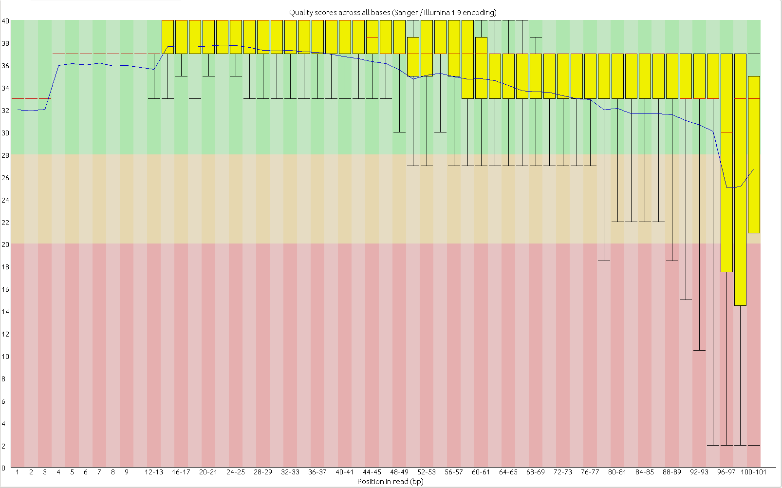
I’ve recalled the SNPs for my Helianthus exilis population genetics for a third time. This time I’m using GATK. This is aligned using BWA to the Nov22k22 reference.
This is two plates of GBS (96-plex each) plus 34 H. annuus samples from G. Baute (also 96-plex GBS). Three exilis samples were removed because they had little or no reads. Reads were trimmed for adapters and quality using trimmomatic (and the number of reads kept after trimming are used here).
So, there is a relationship between number of reads and resulting heterozygosity. It makes some sense because you need a higher number of reads to call a heterozygote than a homozygote. It’s not as bad as what was happening when we were calling snps using the maximum likelihood script. Using a linear model, number of reads accounts for %16 of the variation in heterozygosity.
If you compare this to my previous posts, the heterozygosity is vastly lower for all samples. That is because I previously looked at variable sites with a certain amount of coverage, and here are all sites. So a majority of these sites are invariant.
GBS snp calling
One of the main ways we call SNPs in GBS data is using a maximum likelihood script derived from the original Hohenlohe stickleback RAD paper. It uses a likelihood function based on the number of reads for each base at a site to determine if its homozygous or heterozygous.
It’s been known for a while that it seemed to be biased against high coverage heterozygous sites. I took the script apart and realized that there was actually a serious problem with it. The likelihood function used factorials, and when there were over 175 reads at a site, perl broke down and started describing things as infinite. Then the script would call it as a homozygote by default.
Letting perl work with the huge numbers necessary makes it incredibly slow, so I put in a logic gate for high coverage sites. If there is over 150 reads at a site, and the second most numerous base makes up atleast 10% of the reads (i.e. at minimum 15), then it is heterozygous. Otherwise it is homozygous.
The rest of the script is the same. One could debate how best to call the high coverage scripts, but I suggest you use this script over the old one.
Filtering SNP tables
Previously I posted a pipeline for processing GBS data. At the end of the pipeline, there was a step where the loci were filtered for coverage and heterozygosity. How strict that filtering was could be changed, but it wasn’t obvious in the script and it was slow to rerun. I wrote a new script that takes a raw SNP table (with all sites, including ones with only one individual called) and calculates the stats for each loci. It is then simple and fast to use awk to filter this table for your individual needs. The only filtering the base script does is not print out sites that have four different bases called at the site.