I’ve put together a folder containing information for anyone who may want to continue any of the projects I worked on. I’ve zipped it into a archive called “HandoverDocument_GBaute.zip” and it can be found on /moonriseNFS/ on a external harddrive that I am going to give to Loren and on a couple of thumb drives I am leaving in the lab (one is with my lab notebooks another is in the drawer by Winnies/Megans desk area). You will find information on the seeds, DNA and data used in my thesis and in a number of other projects.
Author Archives: Greg B.
hand emasculation of sunflowers
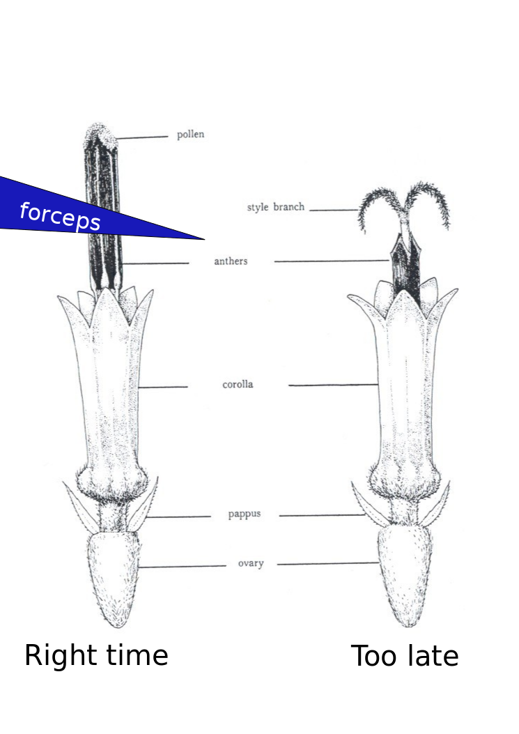
So you want to do some crosses without CMS or relying on self incompatibility? It takes some dedication but it can be done! This is how I carry out hand emasculations. There are hormone based options out there but they can need background specific protocols.
- Grow your plants.
- Bag the heads you want to use when there is 2-3cm between the last leaf and the head. Don’t bag too early and don’t bag too many leaves this will make the head grow crooked.
- Show up ~30 minutes after sunrise or when the greenhouse lights come on. There is variation here with the temperature effecting when the anthers come out of the florets. You can usually figure out the right time to come in a few days. If you show up to early you will only be able to see the very tips of the anthers as the come out of the corolla. These are very difficult to remove. Waiting 15-30 minutes will make a big difference. You will also notices some lines progress at different rates than others.
- Use a set of tweezers like these: http://www.aventools.com/avens-complete-product-line/tools/tweezers-and-quick-test-tweezers/precision-tweezers-1/e-z-pik-precision-tweezers/e-z-pik-tweezers-7-orange#.UzxaJ63c-d8 to remove that days new anthers. See figure for about where and when you should grab the anthers. You can grab a few at a time. You will notice as the morning progresses the pollen at the top of the anther will start to come out and fall all over the place. I find there is about a 1 hour window which is optimal.
- Use a good spray bottle set to a ‘jet’ spray (not mist) and spray down the head. This step is very essential.
- With the head wet inspect it for anther fragments either still in the corolla or fallen down in between florets. Repeat steps 4+5 as needed.
- Repeat steps 3-6 until the flower is done. I find this is about 1 week to ten days for a large cultivar head. If you don’t want to wait for the every floret you can use the forceps or a knife to remove the center florets.
Using LyX to format a thesis for UBC
I used LyX to format my thesis. I started using a set of files made available at the FOGS website. LyX is a “what you see is what you want” interface for Latex. Overall, I had a good experience using this program. There was only one formatting problem in the LyX files online which is now corrected. Other than that I the only things I had to address were errors of my own (too many words in the abstract for example). For sharing, I found it came out looking the nicest to export an HTML file, open it in a browser and then copy pasting it into word. This is a little tedious but I found it was an acceptable trade off given 1) the ease of use 2) how pretty it turned out and 3) the fact that word would have a complete meltdown with this many figures/tables/references. There are plugins for LyX which should allow more direct exporting.
Please let me know if you are able, or unable to use this. If you find and fix bugs please share!
Minimal_Functional_UBC_LyXThesis
Protip: put this folder in dropbox. Use relative paths to all of you figures (which you have put in the figures folder) as I have done in the example. This way you will should be able to generate the pdf from any computer with LyX and dropbox.
How to use FTP (good for uploading data to the SRA)
So you have done everything described in my earlier post about uploading data to the SRA and have received ftp instructions. It is pretty straight forward if you have experience in bash/shell. First navigate into the directory all of your data is in. They type:
ftp ftp-private.ncbi.nlm.nih.gov
Or whatever you target site is. You will be prompted to enter the supplied username and password. From here, the unix commands ‘cd’ ‘ls’ and ‘mkdir’ all work just as on our other machines. You can make a new directory for your data or just dump it where you are (there are no instructions otherwise). To upload one file use ‘put’.
put Myfile1.txt
To a bunch, you should first turn off the prompt and then use mput with a wild card.
prompt
mput MyFile*txt
Check it is all there with ls and leave.
exit
Bibtex library
Even the smartest reference software needs some hand editing help. Here is the bibtex file I used for my thesis. At least the ~200 papers I cite in my thesis are correct. It could be a useful starting point for anyone using a reference manager. The best way to add papers is to find it in google scholar, click cite, click bibtext. Then copy and paste it into this file which you have opened in a plain text editor.
Here it is (you may need to remove the .txt):
Second barcode set
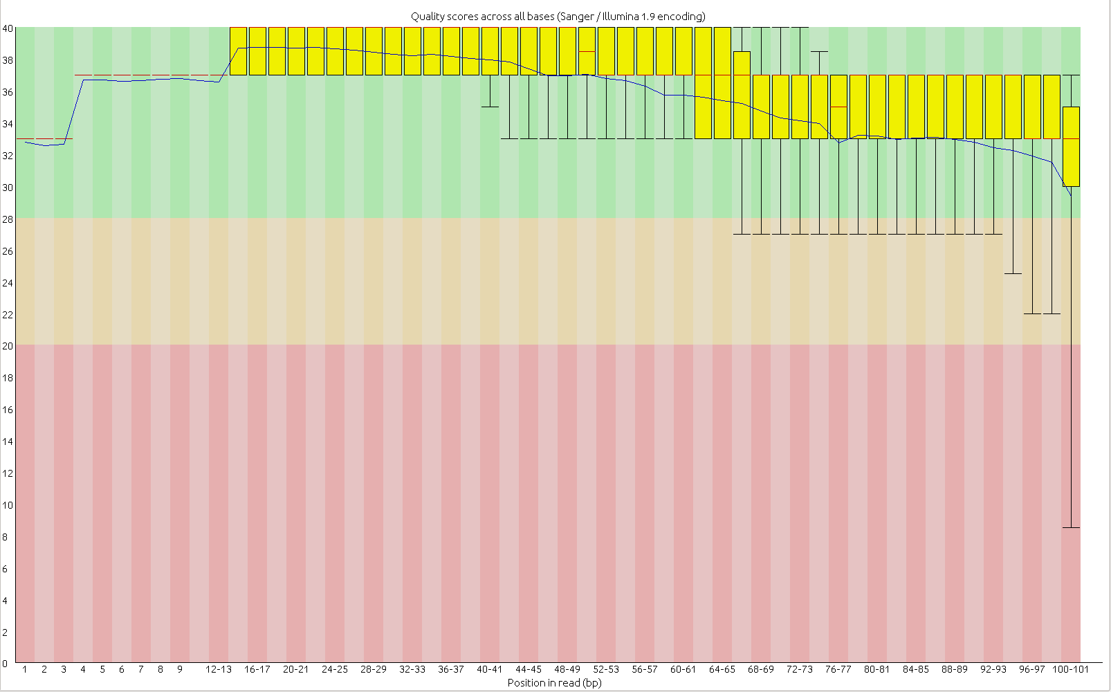
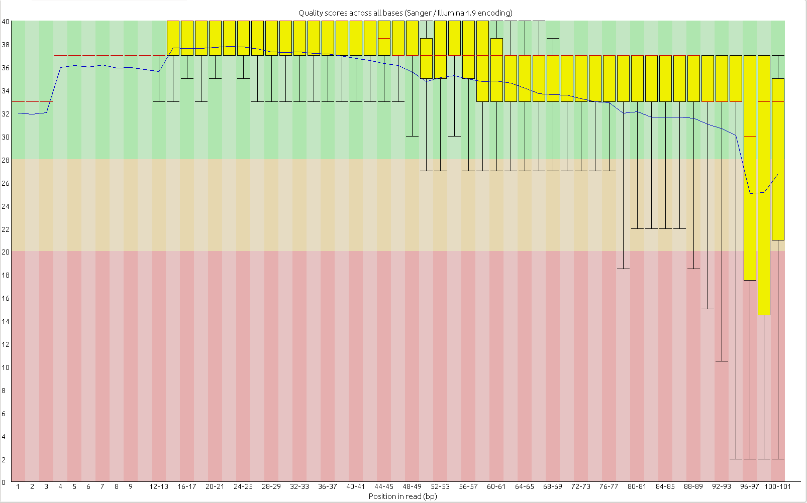
There is now a second set of barcoded adapters that allows higher multiplexing. They also appear to address the quality issues which have been observed in the second read of GBS runs.
This blog post has 1) Info on how to use the barcodes and where they are and 2) some data that might convince you to use them.
Usage
These add a second barcode to the start of the second read before the MSP RE site. The first bases of the second read contain the barcode, just like with the first read. Marco T. designed and ordered these and the info needed to order them is here: https://docs.google.com/spreadsheets/d/1ZXuHKfaR1BYPBX6g0p9GdZHp_21A3z_9pPt_aW0amwM/edit?usp=sharing
I’ve labeled them MTC1-12 and the barcode sequences are as follows.
MTC1 AACT
MTC2 CCAG
MTC3 TTGA
MTC4 GGTCA
MTC5 AACAT
MTC6 CCACG
MTC7 CTTGTA
MTC8 TCGTAT
MTC9 GGACGT
MTC10 AACAGAT
MTC11 CTTGTTA
MTC12 TCGTAAT
They are used in place of the common adapter in the standard protocol (1ul/sample). One possible use, and simplest to use as an example, would be to use these to run 12 plates in a lane. In this case you would make a master mix for the ligation of each plate which contains a different MTC adapter.
Where are they? In the -20 at the back left corner of the bay on the bottom shelf in a box that has a pink lab tape label that says something to the extent of “barcodes + barcoded adapters 1-12”. This contains the working concentration for each of the MTC adapters. Beside that is a box containing the unannealed and as ordered oligos and the annealed stock. The information regarding what I did and what is in the box is written there. The stock needs an additional 1/20 dilution to get to the working concentration
How it looks
First, the quality of the second read is just about as nice as the first read. Using fastqc to look at 4million reads of some random run:
Read one:
Read two:
Now, for the slightly more idiosyncratic part: read counts. In short I dont see any obvious issue with any of these barcodes. I did 5 sets of 5 plates/lane. For all the plates I used the 97-192 bacodes for the Pst side. Then each plate got a differnt MTC barcode for the MSP side. Following the PCR I pooled all of the samples from the plate and quantified. Each plate had a different number of samples which I took into account during the pooling step. Here is the read counts from a randomly selected 4 million reads corrected to number of samples in that plate. Like I said it is a little idiosyncratic but the take home is that they are about as even as you might expect given usual in accuracies in the lab, my hands, and the fact that this is a relatively small sample.
Lane 1
MTC5	14464
MTC1	13518
MTC7	14463
MTC9	13448
MTC3	14232

Lane 2
MTC10	30395
MTC6	11267
MTC2	8263
MTC4	19295
MTC8	14766

Lane 3
MTC5	16631
MTC7	17315
MTC11	11623
MTC9	16256
MTC3	13831

Lane 4
MTC10	11302
MTC6	12120
MTC4	10326
MTC12	18959
MTC8	12832

Lane 5
MTC1	13151
MTC6	13490
MTC2	12851
MTC11	12460
MTC12	17296
Battle of the lids!
Everyone know the foil lids are the undisputed lab champs for normal use and storage. What many people don’t know is that they are more than $2 each! Also, sometimes we can be out and they can be on backorder. Luckily, we have more than 1000 other lids on hand. The problem is that some have bad reputations. Lets find out if they are earned or not!
TLDR: Use Fisherbrand, seal with 75C lid temp.
2 enzyme GBS UNEAK trickery
Want to run UNEAK on a bunch of samples that you sequenced using 2 enzyme GBS? You came to the right place!
This takes R1.fastq.gz and R2.fastq.gz files and makes a single file containing both reads with the appropriate barcodes put on read 2 and the CGG RE site changed to the Pst sequence. This lets you use all of your data in UNEAK… well at least the first 64 bases of all your data!
This also deals with the fact that we get data that is from one lane but split into many files. See example LaneInfo file*. You will also need an appropriately formatted UNEAK key file.
*Only list READ1 in this file. It will only work if your files are named /dir/dir/dir/ABC_R1.fastq.gz and /dir/dir/dir/ABC_R2.fastq.gz.
so the file would read:
/dir/dir/dir/ ABC_R1.fastq C5CDUACXX 3
This is also made to work with .gz fastq files.
usage:
greg@computer$ perl bin/MultiLane_UneakTricker.pl design/UNEAK_KEY_FILE design/LaneInfo.txt /home/greg/project/UNEAK/Illumina
You must have the GBS_Fastq_BarcodeAdder_2Enzyme.pl* in the same bin folder. You also need to make a “tmp” folder.
LaneInfo
MultiLane_UneakTricker_v2
GBS_Fastq_BarcodeAdder_2Enzyme_v2
protip: UNEAK will be fooled by soft links so you can use them instead of copying your data.
Pollination bags
We order our bags here:
http://delstartech.thomasnet.com/viewitems/product-catalog-delnet/delnet-pollination-bags?&plpver=1002&pagesize=200&sortid=&sortorder=asc&forward=&backtoname=
I get 16×18 for annuus heads.
Last time I ordered them they came in 8 days.
BayEnv
Apparently BayEnv is the way to do differentiation scans. Here I offer some scripts and advice to help the you use Bayenv.
Install, no problem get it here: http://gcbias.org/bayenv/ Unzip.
I have to say the documentation is not very good.
There is 2 things you will probably want to use BayEnv for:
1) Environmental correlations
2) XtX population differentiation
I will just be showing XtX here. Both need a covariance matrix. This is not the “matrix.out” file you get from the matrix estimation step.
. But first the SNP table.
Here is a script Greg O made to make a “SNPSFILE”* for bayenv from our standard SNP table format: SNPtable2bayenv I’ve made a small modification so that it excludes any non-bi-allelic site and to also print out a loci info file.
Use it like this:
perl SNPtable2bayenv.pl SNPfile POPfile SampleFile
This will make three files with “SampleFile” appended to the start of the name.
*not actually a SNP file at all, it is an allele count file.
Input SNPfile (all spaces are tabs):
CHROM POS S1 S2 S3 S4 S5
chr1 378627 AA TT NN TT AA
chr2 378661 AA AG NN GG AA
chr3 378746 GG AA NN AA GG
chr4 383246 NN GG NN GG TT
chr5 397421 CC GG NN GG CC
chr6 397424 GG AA NN AA GG
chr7 409691 NN CC NN NN GG
chr8 547653 AA GG NN GG AA
chr9 608412 AA GG NN NN AA
chr10 756412 GG CC NN CC GG
chr11 1065242 NN TT NN NN CC
chr12 1107672 NN TT NN TT NN
POPfile (all spaces are tabs):
S1 p1
S2 p1
S3 p2
S4 p2
...
Now estimate the covarience matrix:
./bayenv2 -i SampleFile.bayenv.txt -p 2 -k 100000 -r21345 > matrix.out
Now this is “matrix.out” file is not what you actually want. You have to use it to make a new file that contains a single covariance matrix. You could use “tail -n3 matrix.out | head -n2 > CovMatrix” or just cut it out yourself. Currently I am just using the last (and hopefully converged) values.
My CovMatrix.txt looks like this (again single tabs between):
3.009807e-05 -1.147699e-07
-1.147699e-07 2.981001e-05
You will also need a environment file. I am not doing the association analysis so am just using some fake data. It is one column for each population and each row is the environmental values. Tab separated.
FakeEnv.txt
1 2
Now you can do the population differentiation test for each snp using a “SNPFILE”. I bet you think you are ready to go? Not so fast, you need a “SNPFILE” not a “SNPSFILE”. Not that either actually really have SNPs in them, just allele counts. Not that I am bitter. SNPFILE is just one site from the SNPSFILE. Here is a script that takes your “SNPSFILE” and runs the XtX program on each of the sites: RunBayenvXtX
perl RunBayenvXtX.pl SampleFile.bayenv.txt SampleFile.LocInfo.txt CovMatrix.txt FakeEnv.txt 2 1
Where 2 is the number of populations and 1 is the number of environmental variables.
This will produce a file that has the site, allelecountfile name and the XtX value.
Paired End for Stacks and UNEAK
Both stacks and uneak are made for single end reads. If you have paired end data here is a little cheat that puts “fake” barcodes onto the mate pairs and prints them all out to one file. It also adds the corresponding fake quality scores.
perl GBS_fastq_RE-multiplexer_v1.pl BarcodeFile R1.fastq R2.fastq Re-barcoded.fastq
BarcodeFile should look like (same as for my demultiplexing script) spaces must be tabs:
sample1 ATCAC
sample2 TGCT
…
# note this could also look like this:
ATCAG ATCAG
TGCT TGCT
…
As it does not actually use the names (it just looks at the second column).
Here it is:
GBS_fastq_RE-multiplexer_v1
actual UNEAK
Some of you may have heard me ramble about my little in house Uneak-like SNP calling approach. I am being converted to using the actual UNEAK pipeline. Why? reason #1 is good god is it fast! I processed 6 lanes raw fastq to snp table in ~1 hour. #2 I am still working on – this will be a comparison of SNP calls between a few methods but I have a good feeling about UNEAK right now.
Here is the UNEAK documentation: http://www.maizegenetics.net/images/stories/bioinformatics/TASSEL/uneak_pipleline_documentation.pdf
It is a little touchy to get it working so I thought I would post so you can avoid these problems.
First install tassel3 (not tassel 4) you will need java 6 or younger to support it: http://www.maizegenetics.net/index.php?option=com_content&task=view&id=89&Itemid=119
To be a hacker turn up the max RAM allocation. Edit run_pipeline.pl to change the line “my $java_mem_max_default = “–Xmx1536m”;” to read something like “my $java_mem_max_default = “–Xmx4g”;” (That is 4g for 4G of RAM).
Go to where you want to do the analysis. This should probably be a new and empty directory. Uneak starts by crawling around looking for fastq files so if the directory has some files you don’t want it using it is going to be unhappy.
Make the directory structure:
../bin/run_pipeline.pl -fork1 -UCreatWorkingDirPlugin -w /home/greg/project/UNEAK/ -endPlugin -runfork1
Move your raw (read: not demultiplexed) fastq or qseq to /Illumina/. If you are using fastq files the names need to look like this: 74PEWAAXX_2_fastq.txt NOT like this:74PAWAAXX_2.fastq and probably not a bunch of other ways. It has to be flow cell name underscore lane number understore fastq dot txt. You might find others work but I know this does (and others don’t).
Make a key file. This is as described in the documentation. It does not have to be complete (every location on the plate) or sorted. Put it in /key/
Flowcell        Lane    Barcode Sample  PlateName       Row     Column
74PEWAAXX       1       CTCGCAAG        425218  MyPlate7        A       1
74PEWAAXX       1       TCCGAAG 425230  MyPlate7        B       1
74PEWAAXX       1       TTCAGA  425242  MyPlate7        C       1
74PEWAAXX       1       ATGATG  425254  MyPlate7        D       1
...
Run it. Barely enough time for coffee.
../bin/tassel3.0_standalone/run_pipeline.pl -fork1 -UFastqToTagCountPlugin -w /home/greg/project/UNEAK/ -e PstI -endPlugin -runfork1
# -c how many times you need to see a tag for it to be included in the network analysis
../bin/tassel3.0_standalone/run_pipeline.pl -fork1 -UMergeTaxaTagCountPlugin -w /home/greg/project/UNEAK/ -c 5 -endPlugin -runfork1
# -e is the "error tolerance rate" although it is not clear to me how this stat is generated
../bin/tassel3.0_standalone/run_pipeline.pl -fork1 -UTagCountToTagPairPlugin -w /home/greg/project/UNEAK/ -e 0.03 -endPlugin -runfork1
../bin/tassel3.0_standalone/run_pipeline.pl -fork1 -UTagPairToTBTPlugin -w /home/greg/project/UNEAK/ -endPlugin -runfork1
../bin/tassel3.0_standalone/run_pipeline.pl -fork1 -UTBTToMapInfoPlugin -w /home/greg/project/UNEAK/ -endPlugin -runfork1
#choose minor and max allele freq
../bin/tassel3.0_standalone/run_pipeline.pl -fork1 -UMapInfoToHapMapPlugin -w /home/greg/project/UNEAK/ -mnMAF 0.01 -mxMAF 0.5 -mnC 0 -mxC 1 -endPlugin -runfork1
fastSTRUCTURE is fast.
fastSTRUCTURE is 2 orders of magnitude faster than structure. For everyone who has waited for structure to run this should make you happy.
Preprint of the manuscript describing it here: http://biorxiv.org/content/early/2013/12/02/001073
UPDATE comparison: Structure_v_FastStructure Structure (top) 8 days and counting FastStructure (below) 15 minutes. You can see the are nearly identical. I would expect them to be within the amount of variation you normally see on structure runs. Structure is only on K=4 (with 50,000 burnin and 100,000 reps and 5 reps of each K) where FastStructure took just under 15 minutes to go K of 1 to 10. Note: these are sorted by Q values not by individuals so, although I think it is highly unlikely, they may be discordant on an individual scale.
UPDATE on speed: ~400 individuals by ~4000 SNPs K=1 to K=10 in just under 15 minutes.
UPDATE on usage: Your structure input file must be labeled .str but in when you call the program leave the .str off. If you don’t adds it itself and will look for MySamples.str.str
It has a few dependencies which can make the installation a little intimidating. I found installing them was relatively easy and I downloaded everything, installed and tested it all in less than one hour.
The site to get fastSTRUCTURE:
http://rajanil.github.io/fastStructure/
You can follow along there, the instructions are pretty good. This is just what I did with a few notes.
At the top you can follow links to the dependencies.
Scipy + Cython
#Scipy
sudo apt-get install python-scipy python-sympy
#Cython
download + scp
tar -zxvf Cython-0.20.tar.gz
cd Cython-0.20/
make
sudo python setup.py install
Numpy
#probably the easiest way:
sudo apt-get install python-numpy python-nose

#what I did before I figured out above:
download + scp
tar -zxvf numpy-1.8.0.tar.gz
cd numpy-1.8.0
python setup.py build --fcompiler=gnu
#also installed "nose" similarly it is at least needed to run the test
#test
python -c 'import numpy; numpy.test()'
On to fastSTRUCTURE
wget --no-check-certificate https://github.com/rajanil/fastStructure/archive/master.tar.gz
#then
#check where GSL is
ls /usr/local/lib
# You should see a bunch of stuff starting with libgsl
# You can look in your LD_LIBRARY_PATH before adding that path
echo $LD_LIBRARY_PATH
# add it
export LD_LIBRARY_PATH=$LD_LIBRARY_PATH:/usr/local/lib
# check it worked
echo $LD_LIBRARY_PATH #mine only has ":/usr/local/lib" in it
#decompress the package
tar -zxvf master.tar.gz
cd fastStructure-master/vars/
python setup.py build_ext --inplace
cd ..
python setup.py build_ext --inplace
#test
python structure.py -K 3 --input=test/testdata --output=testoutput_simple --full --seed=100
GATK on sciborg
A few notes on GATK.
1. GATK requires a younger version of Java than what is on the cluster currently.
> java -jar ./bin/GenomeAnalysisTK-2.8-1-g932cd3a/GenomeAnalysisTK.jar --help Exception in thread "main" java.lang. UnsupportedClassVersionError: org/broadinstitute/sting/gatk/ CommandLineGATK : Unsupported major.minor version 51.0
Get the linux 64 bit version here:
http://java.com/en/download/
move it to sciborg:
> scp ../Downloads/jdk-7u45-linux-x64.tar.gz user@zoology.ubc.ca:cluster/bin/
#ssh  to the cluster extract it:
> tar -zxvf jdk-7u45-linux-x64.tar.gz
#Add it to your path file or use it like so:
> ./bin/jdk1.7.0_45/bin/java -jar ./bin/GenomeAnalysisTK-2.8-1-g932cd3a/GenomeAnalysisTK.jar --help
2. You must have a reference with a relatively small number of contigs/scaffolds
Kay identified and addressed this problem and wrote this script: CombineScaffoldForGATK. I’ve modified it very slightly.
perl CombineScaffoldForGATK.pl GenomeWithManyScaffolds.fa tmp.fa
WARNING: this can print empty lines. The script could be modified to address this but I don’t want to break it. Instead you can fix it with a sed one liner:
sed '/^$/d' tmp.fa > GenomeWith1000Scaffolds.fa
3. You must also prepare the “fasta file”
You also have to index it for BWA with bwa index but GATK needs more, see: http://gatkforums.broadinstitute.org/discussion/1601/how-can-i-prepare-a-fasta-file-to-use-as-reference
In short (in the same dir as your genome):
>java -jar ../bin/picard-tools-1.105/CreateSequenceDictionary.jar R= Nov22k22.split.pheudoScf.fa O= Nov22k22.split.pheudoScf.dict
>samtools faidx Nov22k22.split.pheudoScf.fa
Where does all the GBS data go? Pt. 2
An analysis aimed at addressing some questions generated following discussion of a previous post on GBS…
Number of fragments produced from a ‘digital digestion’ of the Nov22k22 Sunflower assembly:
Clai: 337,793
EcoRI: 449,770
SacI: 242,163
EcoT22I: 528,709
PstI: 129,993
SalI: 1,210,000
HpaII/MspI: 2,755,916
Here is the size distribution of those fragments (omitting fragments of >5000bp):
All the enzymes
With Msp removed for clarity
Take home message: PstI produces fewer fragments of an appropriate size than other enzymes. It looks like the correlation between total number of fragments and number that are the correct size is probably pretty high.
Now for a double digestion. Pst and Msp fragment sizes and again omitting fragments >5000bp. This looks good. In total fragment numbers (also omitting >5000bp fragments):
Pst+Msp total fragments: 187271
Pst+Msp 500<>300bp: 28930
Pst alone total: 79049
Pst alone 500<>300bp:6815
Take home: Two enzyme digestion could work really well. It may yield more than 4 times more usable fragments. I do think we could aim to get even more sites. Maybe some other RE combination could get us to the 100,000 range. With a couple of million reads per sample this could still yield (in an ideal world) 10x at each site. Send me more enzymes sequences and I can do more of the same.
Edited for clarity and changed the post name
Where does all the GBS data go?
Why do we get seemingly few SNPs with GBS data?
Methods: Used bash to count the occurrences of tags. Check your data and let me know what you find:
cat Demutliplexed.fastq | sed -n '2~4p' | cut -c4-70 | sort | uniq -c | grep -v N | sed 's/\s\s*/ /g' > TagCounts
Terminology: I have tried to use tags to refer to a particular sequence and reads as occurrences of those sequences. So a tag may be found 20 times in a sample (20 reads of that sequence).
Findings: Tag repeat distribution
Probably the key thing and a big issue with GBS is the number of times each tag gets sequence. Most sites get sequenced once but most tags get sequence many many times. It is hard to see but here are histograms of the number of times each tags occur for a random sample (my pet11): All tags histogram (note how long the x axis is), 50 tags or less Histogram. Most tags occur once – that is the spike at 1. The tail is long and important. Although only one tag occurs 1088 times it ‘takes up’ 1088 reads.
How does this add up?
In this sample there are 3,453,575 reads. These reads correspond to 376,036 different tag sequences. This would mean (ideally) ~10x depth of each of the tags. This is not the case. There are a mere 718 tags which occur 1000 or more times but they account for 1394905 reads. That is 40% of the reads going to just over 700 (potential) sites. I’ve not looked summarized more samples using the same method but I am sure it would to yield the same result.
Here is an example: Random Deep Tag. Looking at this you can see that the problem is worse than just re-sequencing the same tag many times but you introduce a large number of tags that are sequencing and/or PCR errors that occur once or twice (I cut off many more occurances here).
Conclusion: Poor/incomplete digestion -> few sites get adapters -> they get amplified like crazy and then sequenced.
Update 1:
Of the > 3.4Million tags that are in the set of 18 samples I am playing with only 8123 are in 10 or more of the samples.
For those sites with >10 scored the number of times a tag is sequenced is correlated between samples. The same tags are being sequenced repeatedly in the different samples.
Update 2:
As requested the ‘connectivity’ between tags. This is the number of 1bp miss matches each tag has. To be included in this analysis a tag must occur at least 5 times in 3 individuals. Here is the figure. So most tags have zero matches a smaller number have one and so on. This actually looks pretty good – at least how I am thinking about it now. This could mean that the filtering criteria works. If errors were still being included I would expect tags with one match (the actual sequence) to occur more than ones with zero.
Zoology email forwarding
Hi All,
Here is a link to get your @zoology email to forward to another email (gmail).
https://sun.zoology.ubc.ca:442/cgi-bin/admin/forward.cgi
Use settings (the gear thing in the top right corner) -> accounts -> make default to get gmail to send as your @zoology.
Also, you can use “biodiversity” as an alias for your zoology account. For example:
bob@zoology.ubc.ca is functionally the same as bob@biodiversity.ubc.ca
@botany accounts are completely different.
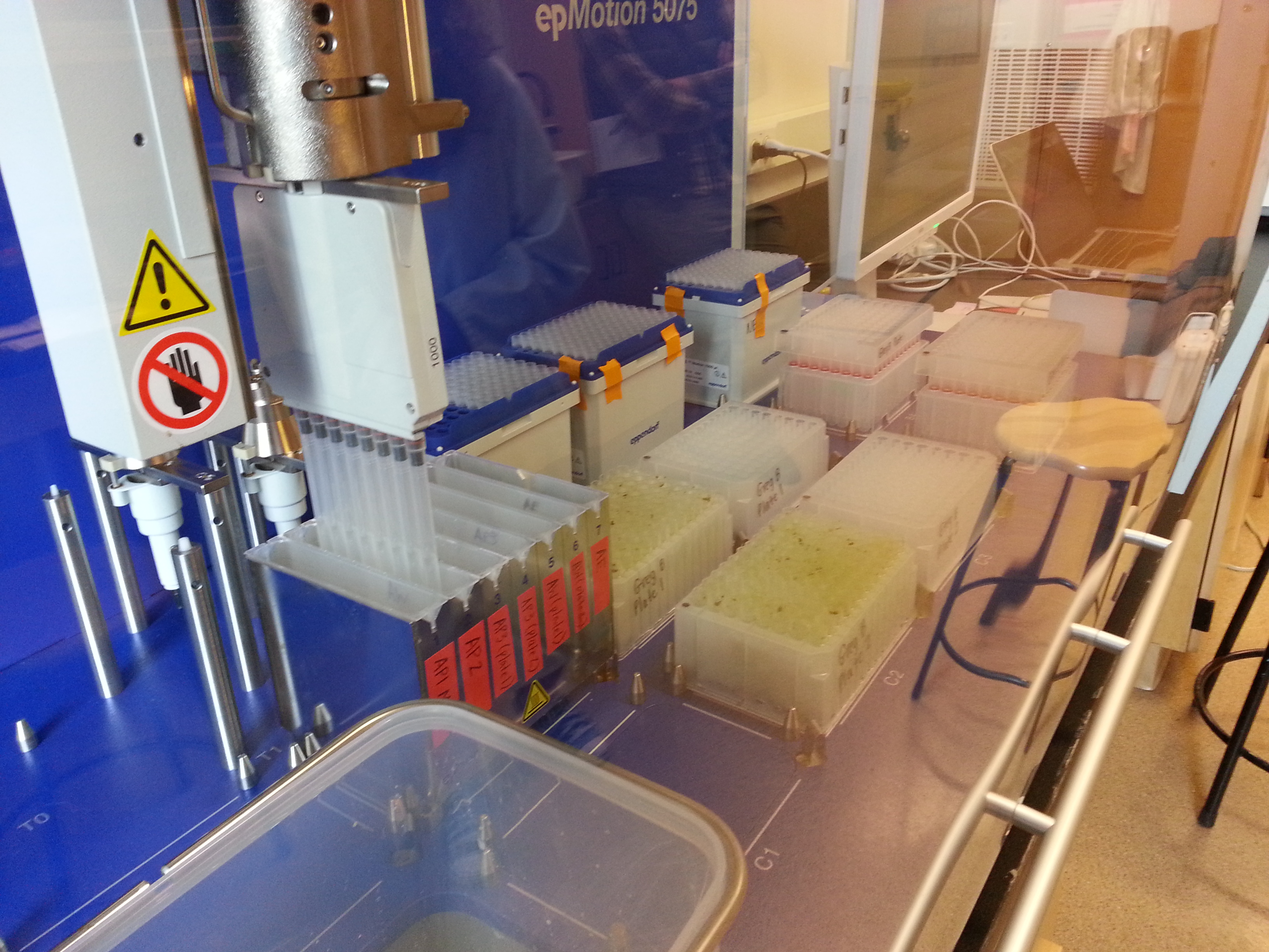
Normalizing DNA with the Robot
Im not looking to volunteer myself as the robot expert, this is just one of the things you need if you are going to use it. These are the files needed to normalize a plate of DNA. One instructs it to take the volumes of DNA from one plate and put them into another and the other is to add the water. I can also offer a poor picture of the machine itself.
GBS multiplexing
GBS_mutliplexing contains 2 scripts that may be useful to you if you are using GBS data. One essentially formats GBS reads for Tassel. The other demultiplexes the reads. A readme file in there explains things in more detail.
Edited: edited the readme and added a script to convert qseq to fastq
Germplasm pedigree
This is a pretty cool figure that is hard to find, I got a hard copy sent to me and scanned it. It is a pedigree of all the publically available lines of sunflower up until 1989. I plan on cleaning this image up and possibly scanning it again, I thought I would save it on here in the mean time. It looks okay if you zoom in.
It is from this paper:
Korell, M., Mosges, G., and Friedt, W., (1992) Construction of a sunflower pedigree map. Helia 15: 7-16