Tag Archives: statistical ecology

On Defining a Statistical Population

The more I do “field ecology” the more I wonder about our standard statistical advice to young ecologists to “random sample your statistical population”. Go to the literature and look for papers on “random environmental fluctuations”, or “non-random processes”, or “random mating” and you will be overwhelmed with references and biology’s preoccupation with randomness. Perhaps we should start with the opposite paradigm, that nothing in the biological world is random in space or time, and then the corollary that if your data show a random pattern or random mating or whatever random, it means you have not done enough research and your inferences are weak.

Since virtually all modern statistical inference rests on a foundation of random sampling, every statistician will be outraged by any concerns that random sampling is possible only in situations that are scientifically uninteresting. It is nearly impossible to find an ecological paper about anything in the real world that even mentions what their statistical “population” is, what they are trying to draw inferences about. And there is a very good reason for this – it is quite impossible to define any statistical population except for those of trivial interest. Suppose we wish to measure the heights of the male 12-year-olds that go to school in Minneapolis in 2017. You can certainly do this, and select a random sample, as all statisticians would recommend. And if you continued to do this for 50 years, you would have a lot of data but no understanding of any growth changes in 12-year-old male humans because the children of 2067 in Minneapolis would be different in many ways from those of today. And so, it is like the daily report of the stock market, lots of numbers with no understanding of processes.

Despite all these ‘philosophical’ issues, ecologists carry on and try to get around this by sampling a small area that is considered homogeneous (to the human eye at least) and then arm waving that their conclusions will apply across the world for similar small areas of some ill-defined habitat (Krebs 2010). Climate change may of course disrupt our conclusions, but perhaps this is all we can do.

Alternatively, we can retreat to the minimalist position and argue that we are drawing no general conclusions but only describing the state of this small piece of real estate in 2017. But alas this is not what science is supposed to be about. We are supposed to reach general conclusions and even general laws with some predictive power. Should biologists just give up pretending they are scientists? That would not be good for our image, but on the other hand to say that the laws of ecology have changed because the climate is changing is not comforting to our political masters. Imagine the outcry if the laws of physics changed over time, so that for example in 25years it might be that CO2 is not a greenhouse gas. Impossible.

These considerations should make ecologists and other biologists very humble, but in fact this cannot be because the media would not approve and money for research would never flow into biology. Humility is a lost virtue in many western cultures, and particularly in ecology we leap from bandwagon to bandwagon to avoid the judgement that our research is limited in application to undefined statistical populations.

One solution to the dilemma of the impossibility of random sampling is just to ignore this requirement, and this approach seems to be the most common solution implicit in ecology papers. Rabe et al. (2002) surveyed the methods used by management agencies to survey population of large mammals and found that even when it was possible to use randomized counts on survey areas, most states used non-random sampling which leads to possible bias in estimates even in aerial surveys. They pointed out that ground surveys of big game were even more likely to provide data based on non-random sampling simply because most of the survey area is very difficult to access on foot. The general problem is that inference is limited in all these wildlife surveys and we do not know the ‘population’ to which the numbers derived are applicable.

In an interesting paper that could apply directly to ecology papers, Williamson (2003) analyzed research papers in a nursing journal to ask if random sampling was utilized in contrast to convenience sampling. He found that only 32% of the 89 studies he reviewed used random sampling. I suspect that this kind of result would apply to much of medical research now, and it might be useful to repeat his kind of analysis with a current ecology journal. He did not consider the even more difficult issue of exactly what statistical population is specified in particular medical studies.

I would recommend that you should put a red flag up when you read “random” in an ecology paper and try to determine how exactly the term is used. But carry on with your research because:

Errors using inadequate data are much less than those using no data at all.

Charles Babbage (1792–1871

Krebs CJ (2010). Case studies and ecological understanding. Chapter 13 in: Billick I, Price MV, eds. The Ecology of Place: Contributions of Place-Based Research to Ecological Understanding. University of Chicago Press, Chicago, pp. 283-302. ISBN: 9780226050430

Rabe, M. J., Rosenstock, S. S. & deVos, J. C. (2002) Review of big-game survey methods used by wildlife agencies of the western United States. Wildlife Society Bulletin, 30, 46-52.

Williamson, G. R. (2003) Misrepresenting random sampling? A systematic review of research papers in the Journal of Advanced Nursing. Journal of Advanced Nursing, 44, 278-288. doi: 10.1046/j.1365-2648.2003.02803.x
 

On Post-hoc Ecology

Back in the Stone Age when science students took philosophy courses, a logic course was a common choice for students majoring in science. Among the many logical fallacies one of the most common was the Post Hoc Fallacy, or in full “Post hoc, ergo propter hoc”, “After this, therefore because of this.” The Post Hoc Fallacy has the following general form:

  1. A occurs before B.
  2. Therefore A is the cause of B.

Many examples of this fallacy are given in the newspapers every day. “I lost my pencil this morning and an earthquake occurred in California this afternoon.” Therefore….. Of course, we are certain that this sort of error could never occur in the 21st century, but I would like to suggest to the contrary that its frequency is probably on the rise in ecology and evolutionary biology, and the culprit (A) is most often climate change.

Hilborn and Stearns (1982) pointed out many years ago that most ecological and evolutionary changes have multiple causes, and thus we must learn to deal with multiple causation in which a variety of factors combine and interact to produce an observed outcome. This point of view places an immediate dichotomy between the two extremes of ecological thinking – single factor experiments to determine causation cleanly versus the “many factors are involved” world view. There are a variety of intermediate views of ecological causality between these two extremes, leading in part to the flow chart syndrome of boxes and arrows aptly described by my CSIRO colleague Kent Williams as “horrendograms”. If you are a natural resource manager you will prefer the simple end of the spectrum to answer the management question of ‘what can I possibly manipulate to change an undesirable outcome for this population or community?’

Many ecological changes are going on today in the world, populations are declining or increasing, species are disappearing, geographical distributions are moving toward the poles or to higher altitudes, and novel diseases are appearing in populations of plants and animals. The simplest explanation of all these changes is that climate change is the major cause because in every part of the Earth some aspect of winter or summer climate is changing. This might be correct, or it might be an example of the Post Hoc Fallacy. How can we determine which explanation is correct?

First, for any ecological change it is important to identify a mechanism of change. Climate, or more properly weather, is itself a complex factor of temperature, humidity, and rainfall, and for climate to be considered a proper cause you must advance some information on physiology or behaviour or genetics that would link some specific climate parameter to the changes observed. Information on possible mechanisms makes the potential explanation more feasible. A second step is to make some specific predictions that can be tested either by experiments or by further observational data. Berteaux et al. (2006) provided a careful list of suggestions on how to proceed in this manner, and Tavecchia et al. (2016) have illustrated how one traditional approach to studying the impact of climate change on population dynamics could lead to forecasting errors.

A second critical focus must be on long-term studies of the population or community of interest. In particular, 3-4 year studies common in Ph.D. theses must make the assumption that the results are a random sample of annual ecological changes. Often this is not the case and this can be recognized when longer term studies are completed or more easily if an experimental manipulation can be carried out on the mechanisms involved.

The retort to these complaints about ecological and evolutionary inference is that all investigated problems are complex and multifactorial, so that after much investigation one can conclude only that “many factors are involved”. The application of AIC analysis attempts to blunt this criticism by taking the approach that, given the data (the evidence), what hypothesis is best supported? Hobbs and Hilborn (2006) provide a guide to the different methods of inference that can improve on the standard statistical approach. The AIC approach has always carried with it the awareness of the possibility that the correct hypothesis is not present in the list being evaluated, or that some combination of relevant factors cannot be tested because the available data does not cover a wide enough range of variation. Burnham et al. (2011) provide an excellent checklist for the use of AIC measures to discriminate among hypotheses. Guthery et al. (2005) and Stephens et al. (2005) carry the discussion in interesting ways. Cade (2015) discusses an interesting case in which inappropriate AIC methods lead to questionable conclusions about habitat distribution preferences and use by sage-grouse in Colorado.

If there is a simple message in all this it is to think very carefully about what the problem is in any investigation, what the possible solutions or hypotheses are that could explain the problem, and then utilize the best statistical methods to answer that question. Older statistical methods are not necessarily bad, and newer statistical methods not automatically better for solving problems. The key lies in good data, relevant to the problem being investigated. And if you are a beginning investigator, read some of these papers.

Berteaux, D., et al. 2006. Constraints to projecting the effects of climate change on mammals. Climate Research 32(2): 151-158. doi: 10.3354/cr032151.

Burnham, K.P., Anderson, D.R., and Huyvaert, K.P. 2011. AIC model selection and multimodel inference in behavioral ecology: some background, observations, and comparisons. Behavioral Ecology and Sociobiology 65(1): 23-35. doi: 10.1007/s00265-010-1029-6.

Guthery, F.S., Brennan, L.A., Peterson, M.J., and Lusk, J.J. 2005. Information theory in wildlife science: Critique and viewpoint. Journal of Wildlife Management 69(2): 457-465. doi: 10.1890/04-0645.

Hilborn, R., and Stearns, S.C. 1982. On inference in ecology and evolutionary biology: the problem of multiple causes. Acta Biotheoretica 31: 145-164. doi: 10.1007/BF01857238

Hobbs, N.T., and Hilborn, R. 2006. Alternatives to statistical hypothesis testing in ecology: a guide to self teaching. Ecological Applications 16(1): 5-19. doi: 10.1890/04-0645

Stephens, P.A., Buskirk, S.W., Hayward, G.D., and Del Rio, C.M. 2005. Information theory and hypothesis testing: a call for pluralism. Journal of Applied Ecology 42(1): 4-12. doi: 10.1111/j.1365-2664.2005.01002.x

Tavecchia, G., et al. 2016. Climate-driven vital rates do not always mean climate-driven population. Global Change Biology 22(12): 3960-3966. doi: 10.1111/gcb.13330.

On Indices of Population Abundance

A discussion with Murray Efford last week stimulated me to raise again this issue of using indices to measure population changes. One could argue that this issue has already been fully aired by Anderson (2003) and Engemann (2003) and I discussed it briefly in a blog about 2 years ago. The general agreement appears to be that mark-recapture estimation of population size is highly desirable if the capture procedure is clearly understood in relation to the assumption of the model of estimation. McKelvey and Pearson (2001) made this point with some elegant simulations. The best procedure then, if one wishes to replace mark-recapture methods with some index of abundance (track counts, songs, fecal pellets, etc.), is to calibrate the index with absolute abundance information of some type and show that the index and absolute abundance are very highly correlated. This calibration is difficult because there are few natural populations on which we know absolute abundance with high accuracy. We are left hanging with no clear path forward, particularly for monitoring programs that have little time or money to do extensive counting of any one species.

McKelvey and Pearson (2001) laid out a good guide for the use of indices in small mammal trapping, and showed that for many sampling programs the use of the number of unique individuals caught in a sampling session was a good index of population abundance, even though it is negatively biased. The key variable in all these discussions of mark-recapture models is the probability of capture of an individual animal living on the trapping area per session. Many years ago Leslie et al. (1953) considered this issue and the practical result was the recommendation that all subsequent work with small rodents should aim for a maximum probability of capture of individuals. The simplest way to do this was with highly efficient traps and large numbers of traps (single catch traps) so that there was always an excess of traps available for the population being censused. Krebs and Boonstra (1984) presented an analysis of trappability for several Microtus populations in which these recommendations were typically followed (Longworth traps in excess), and they found that the average per session detection probability ranged from about 0.6 to 0.9 for the four Microtus species studied. In all these studies live traps were present year round in the field, locked open when not in use, so the traps became part of the local environment for the voles. Clean live traps were much less likely to catch Microtus townsendii than dirty traps soiled with urine and feces (Boonstra and Krebs 1976). It is clear that minor behavioural quirks of the species under study may have significant effects on the capture data obtained. Individual heterogeneity in the probability of capture is a major problem in all mark-recapture work. But in the end natural history is as important as statistics.

There are at least two take home messages that can come from all these considerations. First, there are many statistical decisions that have to be made before population size can be estimated from mark-recapture data or any kind of quadrat based data. Second, there is also much biological information that must be well known before starting out with some kind of sampling design. Detectability may vary greatly with observers, with types of traps used, and observer skills so that again the devil is in the details. A third take home message given to me by someone who must remain nameless is that mark-recapture is hopeless as an ecological method because even after much work, the elusive population size that one wishes to know is lost in a pile of assumptions. But we cannot accept such a negative view without trying very hard to overcome the problems of sampling and estimation.

One way out of the box we find ourselves in (if we want to estimate population size) is to use an index of abundance and recognize its limitations. We cannot use quantitative population modelling on indices but we may find that indices are the best we can do for now. In particular, monitoring with little money must rely on indices of many populations of both plants and animals. Some data are better than no data for the management of populations and communities.

For the present time spatially explicit capture-recapture (SECR) methods of population estimation have provided a most useful approach to estimating density (Efford et al. 2009, 2013) and much future work will be needed to tell us how useful this relatively new approach is for accurately estimating population density (Broekhuis and Gopalaswamy 2016).

And a final reminder that even if you study community or ecosystem ecology, you must rely on getting measures of abundance for many quantitative models of system performance. So methods that provide accuracy for population sizes are just as essential for the vast array of ecological studies.

Anderson, D.R. 2003. Index values rarely constitute reliable information. Wildlife Society Bulletin 31(1): 288-291.

Boonstra, R. and Krebs, C.J. 1976. The effect of odour on trap response in Microtus townsendii. Journal of Zoology (London) 180(4): 467-476. Doi: 10.1111/j.1469-7998.1976.tb04692.x.

Broekhuis, F. and Gopalaswamy, A.M. 2016. Counting cats: Spatially explicit population estimates of cheetah (Acinonyx jubatus) using unstructured sampling data. PLoS ONE 11(5): e0153875. Doi: 10.1371/journal.pone.0153875.

Efford, M.G. and Fewster, R.M. 2013. Estimating population size by spatially explicit capture–recapture. Oikos 122(6): 918-928. Doi: 10.1111/j.1600-0706.2012.20440.x.

Efford, M.G., Dawson, D.K., and Borchers, D.L. 2009. Population density estimated from locations of individuals on a passive detector array. Ecology 90(10): 2676-2682. Doi: 10.1890/08-1735.1

Engeman, R.M. 2003. More on the need to get the basics right: population indices. Wildlife Society Bulletin 31(1): 286-287.

Krebs, C.J. and Boonstra, R. 1984. Trappability estimates for mark-recapture data. Canadian Journal of Zoology 62 (12): 2440-2444. Doi: 10.1139/z84-360

Leslie, P.H., Chitty, D., and Chitty, H. 1953. The estimation of population parameters from data obtained by means of the capture-recapture method. III. An example of the practical applications of the method. Biometrika 40 (1-2): 137-169. Doi:10.1093/biomet/40.1-2.137

McKelvey, K.S. & Pearson, D.E. (2001) Population estimation with sparse data: the role of estimators versus indices revisited. Canadian Journal of Zoology, 79(10): 1754-1765. Doi: 10.1139/cjz-79-10-1754

On Statistical Progress in Ecology

There is a general belief that science progresses over time and given that the number of scientists is increasing, this is a reasonable first approximation. The use of statistics in ecology has been one of ever increasing improvements of methods of analysis, accompanied by bandwagons. It is one of these bandwagons that I want to discuss here by raising the general question:

Has the introduction of new methods of analysis in biological statistics led to advances in ecological understanding?

This is a very general question and could be discussed at many levels, but I want to concentrate on the top levels of statistical inference by means of old-style frequentist statistics, Bayesian methods, and information theoretic methods. I am prompted to ask this question because of my reviewing of many papers submitted to ecological journals in which the data are so buried by the statistical analysis that the reader is left in a state of confusion whether or not any progress has been made. Being amazed by the methodology is not the same as being impressed by the advance in ecological understanding.

Old style frequentist statistics (read Sokal and Rohlf textbook) has been criticized for concentrating on null hypothesis testing when everyone knows the null hypothesis is not correct. This has led to refinements in methods of inference that rely on effect size and predictive power that is now the standard in new statistical texts. Information-theoretic methods came in to fill the gap by making the data primary (rather than the null hypothesis) and asking the question which of several hypotheses best fit the data (Anderson et al. 2000). The key here was to recognize that one should have prior expectations or several alternative hypotheses in any investigation, as recommended in 1897 by Chamberlin. Bayesian analysis furthered the discussion not only by having several alternative hypotheses but by the ability to use prior information in the analysis (McCarthy and Masters 2006). Implicit in both information theoretic and Bayesian analysis is the recognition that all of the alternative hypotheses might be incorrect, and that the hypothesis selected as ‘best’ might have very low predictive power.

Two problems have arisen as a result of this change of focus in model selection. The first is the problem of testability. There is an implicit disregard for the old idea that models or conclusions from an analysis should be tested with further data, preferably with data obtained independently from the original data used to find the ‘best’ model. The assumption might be made that if we get further data, we should add it to the prior data and update the model so that it somehow begins to approach the ‘perfect’ model. This was the original definition of passive adaptive management, which is now suggested to be a poor model for natural resource management. The second problem is that the model selected as ‘best’ may be of little use for natural resource management because it has little predictability. In management issues for conservation or exploitation of wildlife there may be many variables that affect population changes and it may not be possible to conduct active adaptive management for all of these variables.

The take home message is that we need in the conclusions of our papers to have a measure of progress in ecological insight whatever statistical methods we use. The significance of our research will not be measured by the number of p-values, AIC values, BIC values, or complicated tables. The key question must be: What new ecological insights have been achieved by these methods?

Anderson, D.R., Burnham, K.P., and Thompson, W.L. 2000. Null hypothesis testing: problems, prevalence, and an alternative. Journal of Wildlife Management 64(4): 912-923.

Chamberlin, T.C. 1897. The method of multiple working hypotheses. Journal of Geology 5: 837-848 (reprinted in Science 148: 754-759 in 1965). doi:10.1126/science.148.3671.754.

McCarthy, M.A., and Masters, P.I.P. 2005. Profiting from prior information in Bayesian analyses of ecological data. Journal of Applied Ecology 42(6): 1012-1019. doi:10.1111/j.1365-2664.2005.01101.x.

Walters, C. 1986. Adaptive Management of Renewable Resources. Macmillan, New York.


What do the Data Points Mean?

In Statistics 101 we were told that each data point in a scatter plot should have a precise meaning. Hopefully all ecologists agree with this, and if so I proceed to ask two questions about the ecology literature:

  1. What fraction of scatter plots in ecology papers define what the dots on the plot mean? Are they individual measurements, are they means of several measurements? Are they predictions from a mathematical model?
  2. Given that we know what the dots are, are we shown confidence limits for the points, or do we assume they are absolutely precise with no possible error?

With these two simple questions in mind I did a short, non-random search of recent ecology journals. Perhaps if a graduate ecology class is reading this blog, they could do a much wider search so that we might even be able to tell some of the editors of our journals how they score on Statistics 101 Quiz # 1. I went through 3 issues of Ecology (2015, issues 4, 5, and 6), 3 issues of the Journal of Animal Ecology (2015, issues 4 to 6), and 3 issues of Ecology Letters (2016, issues 1, 2, and 3). I scored each figure in each paper. The first question above is harder to score, so I divided the answer into three groups: clearly defined in figure legend, not defined in figure legend but clear in the paper itself, and not clearly defined anywhere. I kept the second question above on a simpler scale by asking if there were or were not confidence limits or S.E. on the dots in the scatter diagram. I considered histogram bars as ‘data points’ equivalent to scatter plots and scored these with these same 2 questions. I scored figures with multiple plots in the same figure as just one data source for my survey. I ignored maps, simulation data, and papers with only models. I got these results:

    Data points Confidence Limits or S.E.
Journal Number of papers Clearly defined in figure legend Yes No
Ecology 80 179
(95%)
98
(50%)
96
(50%)
Journal of Animal Ecology 84 195
(98%)
119
(60%)
81
(40%)
Ecology Letters 33 64
(94%)
29
(43%)
39
(57%)

The good news is that virtually all the data points in figures that contained empirical data were clearly defined, so the first question was not problematic. The potentially bad news is that around half of the data figures did not contain any measure of statistical precision for the data points.

There could be many reasons why confidence limits could not be applied to data points on graphs in papers. In some cases it would clutter the plot too much. In other cases the data points are completely accurate and have no error although this might be unusual in ecological data. Whatever the reason, some mention of the reason should be given in the text or the figure legend.

There were many limitations to this brief survey. It is clear that some subdisciplines of ecology adhere to Statistics 101 recommendations more carefully than others, but I did not tally these subdisciplines. One could make a thesis out of this sort of tally. Often I could not decipher if the data point was for an experimental unit or for a sampling unit but I have not analyzed for this error here.

So what do we conclude from this non-random survey? The take home message for authors is to make sure that the data points or histograms in their published figures are clearly defined in the figure legend and include if possible some measure of probable error. The message for reviewers and journal editors is to check that data points presented in submitted papers are properly identified and labeled with some measure of precision.

On Log-Log Regressions

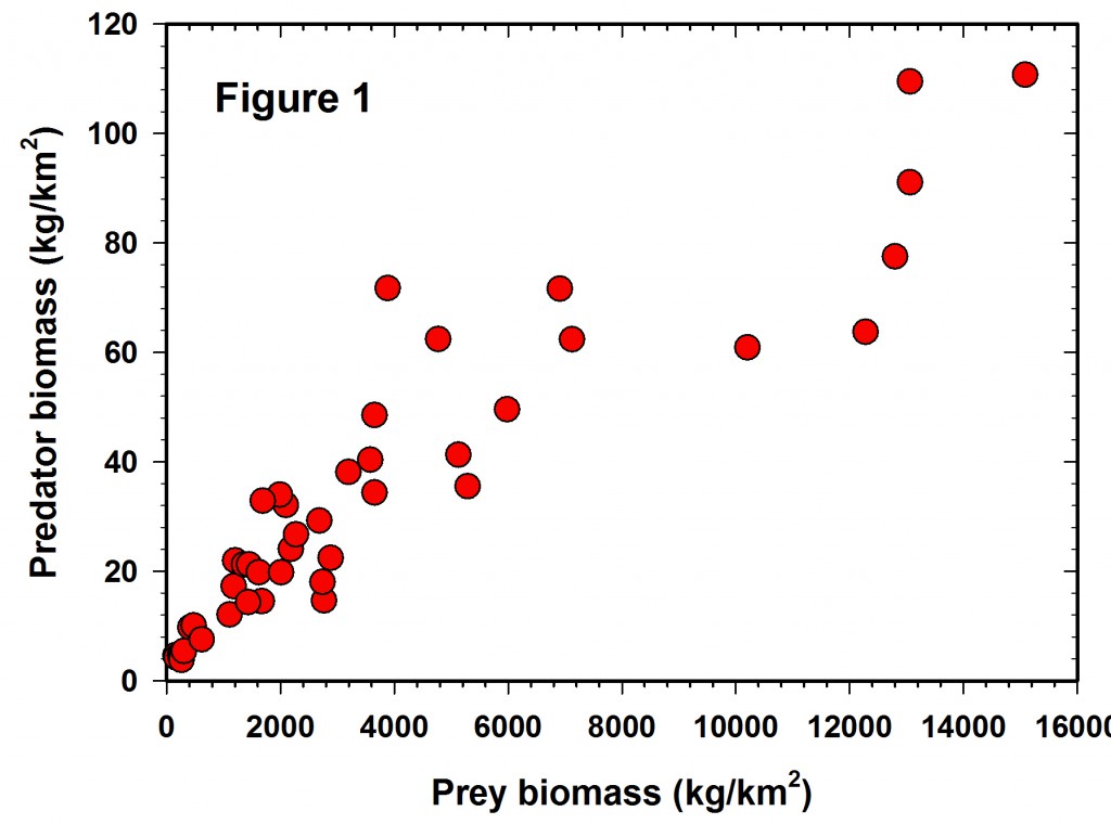
Log-log regressions are commonly used in ecological papers, and my attention to their limitations was twigged by a recent paper by Hatton et al. (2015) in Science. I want to look at just one example of a log-log regression from this paper as an illustration of what I think might be some pitfalls of this approach. The regression under discussion is Figure 1 in the Hatton paper, a plot of predator biomass (Y) on prey biomass (X) for a variety of African large mammal ecosystems. I emphasize that this is a critique of log-log regression problems, not a detailed critique of this paper.

Figure 1 shows the raw data reported in the Hatton et al. (2015) paper but plotted in arithmetic space. It is clear that the variance increases with the mean and the data are highly variable, as well as slightly curvilinear, so a transformation is clearly desirable for statistical analysis. Unfortunately we are given no error bars on each of the point estimates, so it is not possible to plot confidence limits for each estimate.

Figure 1A

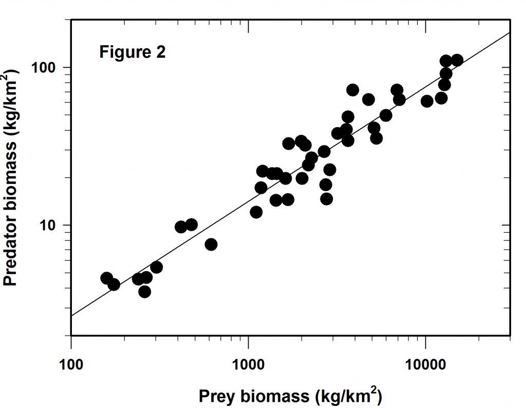
We log both the axes and get Figure 2 which is identical to that plotted as Figure 1 in Hatton et al. (2015). Clearly the regression fit is better that that of Figure 1 and yet there is still considerable variation around the line of best fit.

Figure 2A

The variation around this log-log line is the main issue I wish to discuss here. Much depends on the reason for the regression line. Mac Nally (2000) made the point that regressions are often used for predictive purposes but sometimes used only as explanations. I assume here one wishes this to be a predictive regression.

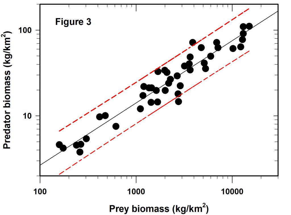
So the next question is if the Figure 2 regression is predictive, how wide are the confidence limits? In this case we will adopt the usual 95% confidence predictions for a single data point. The result is shown in Figure 3, which did not appear in the Science article. The red lines define the 95% confidence belt.

Figure 3A

Now comes the main point of my concerns with log-log regressions. What do these error limits really mean when they are translated back to the original measurements that define the graph?

The table given below gives the prediction intervals for a hypothetical set of 8 prey abundances scattered along the span of prey densities reported.

Prey abundance (kg/km2)

Estimated predator abundance (kg/km2)

Predicted lower 95% confidence limit

Predicted upper 95% confidence limit

Width of lower confidence interval (%)

Width of upper confidence interval (%)

200

4.4

2.46

7.74

-44%

+76%

1000

14.1

8.16

24.6

-42%

+74%

1500

19.0

11.0

33.2

-42%

+70%

2000

23.4

13.2

41.0

-44%

+75%

4000

38.7

22.4

69.0

-42%

+78%

8000

64.0

35.4

113.6

-45%

+78%

10000

75.2

43.6

134.4

-42%

+79%

12000

85.8

49.0

147.6

-43%

+72%

The overall average confidence limits for this log-log regression are -43% to +75%, given that the SE of the predictions varies little across the range of values used in the regression. These are very broad confidence limits for any prediction from a regression line.

The bottom line is that log-log regressions can camouflage a great deal of variation, which may or may not be acceptable depending on the use of the regression. These plots always visually look much better than they are. You probably already knew this but I worry that it is a point that can be easily overlooked.

Lastly, a minor quibble with this regression. Some authors (e.g. Ricker 1983, Smith 2009) have discussed the issue of using the reduced major axis (or geometric mean regression) when the X variable is measured with error instead of the standard regression method. One could argue for this particular data set that the X variable is measured with error, so that I have used a reduced major axis regression in this discussion. The overall conclusions are not changed if standard regression methods are used.

Hatton, I.A., McCann, K.S., Fryxell, J.M., Davies, T.J., Smerlak, M., Sinclair, A.R.E. & Loreau, M. (2015) The predator-prey power law: Biomass scaling across terrestrial and aquatic biomes. Science 349 (6252). doi: 10.1126/science.aac6284

Mac Nally, R. (2000) Regression and model-building in conservation biology, biogeography and ecology: The distinction between – and reconciliation of – ‘predictive’ and ‘explanatory’ models. Biodiversity & Conservation, 9, 655-671. doi: 10.1023/A:1008985925162

Ricker, W.E. (1984) Computation and uses of central trend lines. Canadian Journal of Zoology 62 (10), 1897-1905.doi: 10.1139/z84-279

Smith, R.J. (2009) Use and misuse of the reduced major axis for line-fitting. American Journal of Physical Anthropology, 140, 476-486. doi: 10.1002/ajpa.21090

On Repeatability in Ecology

One of the elementary lessons of statistics is that every measurement must be repeatable so that differences or changes in some ecological variable can be interpreted with respect to some ecological or environmental mechanism. So if we count 40 elephants in one year and count 80 in the following year, we know that population abundance has changed and we do not have to consider the possibility that the repeatability of our counting method is so poor that 40 and 80 could refer to the same population size. Both precision and bias come into the discussion at this point. Much of the elaboration of ecological methods involves the attempt to improve the precision of methods such as those for estimating abundance or species richness. There is less discussion of the problem of bias.

The repeatability that is most crucial in forging a solid science is that associated with experiments. We should not simply do an important experiment in a single place and then assume the results apply world-wide. Of course we do this, but we should always remember that this is a gigantic leap of faith. Ecologists are often not willing to repeat critical experiments, in contrast to scientists in chemistry or molecular biology. Part of this reluctance is understandable because the costs associated with many important field experiments is large and funding committees must then judge whether to repeat the old or fund the new. But if we do not repeat the old, we never can discover the limits to our hypotheses or generalizations. Given a limited amount of money, experimental designs often limit the potential generality of the conclusions. Should you have 2 or 4 or 6 replicates? Should you have more replicates and fewer treatment sites or levels of manipulation? When we can, we try one way and then another to see if we get similar results.

A looming issue now is climate change which means that the ecosystem studied in 1980 is possibly rather different than the one you now study in 2014, or the place someone manipulated in 1970 is not the same community you manipulated this year. The worst case scenario would be to find out that you have to do the same experiment every ten years to check if the whole response system has changed. Impossible with current funding levels. How can we develop a robust set of generalizations or ‘theories’ in ecology if the world is changing so that the food webs we so carefully described have now broken down? I am not sure what the answers are to these difficult questions.

And then you pile evolution into this mix and wonder if organisms can change like Donelson et al.’s (2012) tropical reef fish, so that climate changes might be less significant than we currently think, at least for some species. The frustration that ecologists now face over these issues with respect to ecosystem management boils over in many verbal discussions like those on “novel ecosystems” (Hobbs et al. 2014, Aronson et al. 2014) that can be viewed as critical decisions about how to think about environmental change or a discussion about angels on pinheads.

Underlying all of this is the global issue of repeatability, and whether our current perceptions of how to manage ecosystems is sufficiently reliable to sidestep the adaptive management scenarios that seem so useful in theory (Conroy et al. 2011) but are at present rare in practice (Keith et al. 2011). The need for action in conservation biology seems to trump the need for repeatability to test the generalizations on which we base our management recommendations. This need is apparent in all our sciences that affect humans directly. In agriculture we release new varieties of crops with minimal long term studies of their effects on the ecosystem, or we introduce new methods such as no till agriculture without adequate studies of its impacts on soil structure and pest species. This kind of hubris does guarantee long term employment in mitigating adverse consequences, but is perhaps not an optimal way to proceed in environmental management. We cannot follow the Hippocratic Oath in applied ecology because all our management actions create winners and losers, and ‘harm’ then becomes an opinion about how we designate ‘winners’ and ‘losers’. Using social science is one way out of this dilemma, but history gives sparse support for the idea of ‘expert’ opinion for good environmental action.

Aronson, J., Murcia, C., Kattan, G.H., Moreno-Mateos, D., Dixon, K. & Simberloff, D. (2014) The road to confusion is paved with novel ecosystem labels: a reply to Hobbs et al. Trends in Ecology & Evolution, 29, 646-647.

Conroy, M.J., Runge, M.C., Nichols, J.D., Stodola, K.W. & Cooper, R.J. (2011) Conservation in the face of climate change: The roles of alternative models, monitoring, and adaptation in confronting and reducing uncertainty. Biological Conservation, 144, 1204-1213.

Donelson, J.M., Munday, P.L., McCormick, M.I. & Pitcher, C.R. (2012) Rapid transgenerational acclimation of a tropical reef fish to climate change. Nature Climate Change, 2, 30-32.

Hobbs, R.J., Higgs, E.S. & Harris, J.A. (2014) Novel ecosystems: concept or inconvenient reality? A response to Murcia et al. Trends in Ecology & Evolution, 29, 645-646.

Keith, D.A., Martin, T.G., McDonald-Madden, E. & Walters, C. (2011) Uncertainty and adaptive management for biodiversity conservation. Biological Conservation, 144, 1175-1178.