
Parameters:
Description: The binomial distribution gives the probability of having k "successes" in n trials.
Parameters:
Description: The geometric distribution gives the probability that the first successful trial will be the k one. That is, there will be (k-1) unsuccessful trials followed by a successful one.
Description: Similar to the geometric distribution, except that the negative binomial distribution describes the number of trials until the rth success.
Parameters:
 = mean number
Description: The Poisson distribution gives the number of events in a given time period when the events occur randomly and are independent of one another (= Poisson arrival process). Similarly, the Poisson distribution gives the number of events in a given area when the presence or absence of a point is independent of occurrences at other points (= Poisson random scatter).
Sources: The binomial distribution approaches a Poisson distribution when p is small.
A continuous distribution describes the density of events in a particular region along a continuous axis (like the real line).
Continuous distributions are described by density functions, f(x). Integrating a density function from points a to b gives the probability that a random variable X will fall between these points.
Parameters:
= mean of the distribution
 = standard deviation of the distribution
Description: The normal distribution has a bell-shaped density function.
Sources: "Roughly, the central limit theorem says that if a random variable is the sum of a large number of independent random variables, it is approximately normally distributed" (Rice p.51). For example, the normal distribution is a good fit to the binomial distribution with p=1/2 after about 30 trials.
Parameters:
 = the rate at which events occur
Description: The exponential distribution gives the distribution of the time until the first event. This is often called the lifetime of the process (when the event is death or malfunction).
Sources: The exponential distribution describes the time between arrivals in a Poisson arrival process which occurs at rate .
The exponential distribution also approximates the geometric distribution when p is small (Note: they then have the same mean and variance).
Description: Similar to the exponential distribution, except that the gamma distribution describes the time until  events have occurred.
Assume that there are N haploid individuals in a population (constant over time!).
(WARNING: Hudson counts N haploid individuals. Tajima counts N diploid individuals for a total of 2N alleles.)
N offspring are chosen from the N parents randomly with replacement.
The number of offspring of Parent #1, say, follows a binomial distribution with p=1/N. On average, this parent will have N p =1 offspring with variance N p (1-p) ~ 1.
Since p is small, the number of offspring per parent is approximately Poisson distributed with =1.
The probability that two individuals will have the same parent is 1/N. This is called a "coalescent event": two alleles in the current generation trace back to a single allelic copy in the previous generation.
For n individuals to each have different parents in the previous generation, the second allele has to have a different parent (Prob=1-1/N), the third parent has to have a different allele from either the first or the second (Prob=1-2/N), etc:
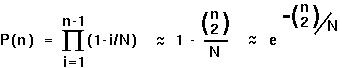
P(n) is the probability that there will not be a coalescent event in the previous generation in a sample of n alleles.
(Following Hudson 1990).
Coalescent processes work backwards in time, from the current generation (0) back t generations.
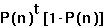
If in each generation, the probability that there is not a coalescent event is P(n), then the expected time until the first "success" (ie first coalescent) follows a geometric distribution:
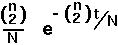
If the probability of a coalescent event, 1-P(n), is small, then this distribution may be approximated by the exponential distribution:
That is, the expected time until the first coalescent event is simply
 .
.
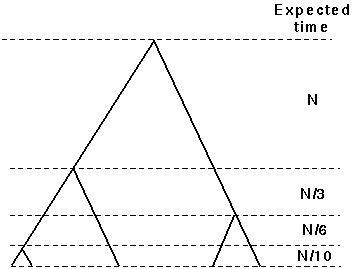
This is extremely useful. For instance, we can use it to find the expected time until the last coalescent event:
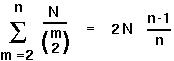 .
.
The time it takes for a sample of 2 alleles to coalesce is about N generations. For 3 alleles, it takes on average 4/3 N generations. And for many alleles in the sample it takes about 2N (in the haploid model; 4N in the diploid model).
 .
.
This illustrates cool facts about the coalescent process:
Key assumptions: The population remains constant, with the number of offspring per parent following a Poisson distribution.
To the extent (!!) that these assumptions apply to species lineages (not just allelic lineages within a population), the coalescent can also be used to describe phylogenetic trees of species.
At a coalescent event, each pair of lineages is equally likely to coalesce.
This fact can be used to generate the probability of any particular tree topology (see Tajima 1983).
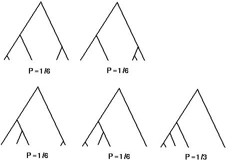
One point Tajima makes is that it is reasonably likely for such trees to look assymetrical.
For instance, in an n allele tree, the probability that the one lineage is very different from all the rest (as in the last two diagrams) is 2/(n-1) (=1/2 in the diagram).
Knowing the distribution of branch lengths and the probability of different tree topologies, one can make inferences about the extent of sequence divergence expected in a given sample.
For example, the number of segregating sites expected in a sample (S) is the mutation rate per sequence length per generation () times the total length of all the branches of a tree:
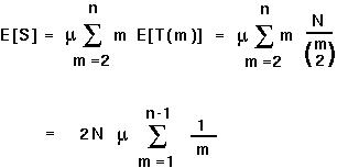
For example, with a sample of 2 sequences (n=2), we would expect
2 N sites to vary between the two sequences.
Conversely, if 2 N is unknown, it can be estimated as the number of segregating sites in a sample of two sequences from a population.
The power of coalescent theory is that one can obtain the expected value of properties (like the number of segregating sites in a sample) and compare the observed property against this expectation.
 Back to biology 500D home page.