Log-log regressions are commonly used in ecological papers, and my attention to their limitations was twigged by a recent paper by Hatton et al. (2015) in Science. I want to look at just one example of a log-log regression from this paper as an illustration of what I think might be some pitfalls of this approach. The regression under discussion is Figure 1 in the Hatton paper, a plot of predator biomass (Y) on prey biomass (X) for a variety of African large mammal ecosystems. I emphasize that this is a critique of log-log regression problems, not a detailed critique of this paper.

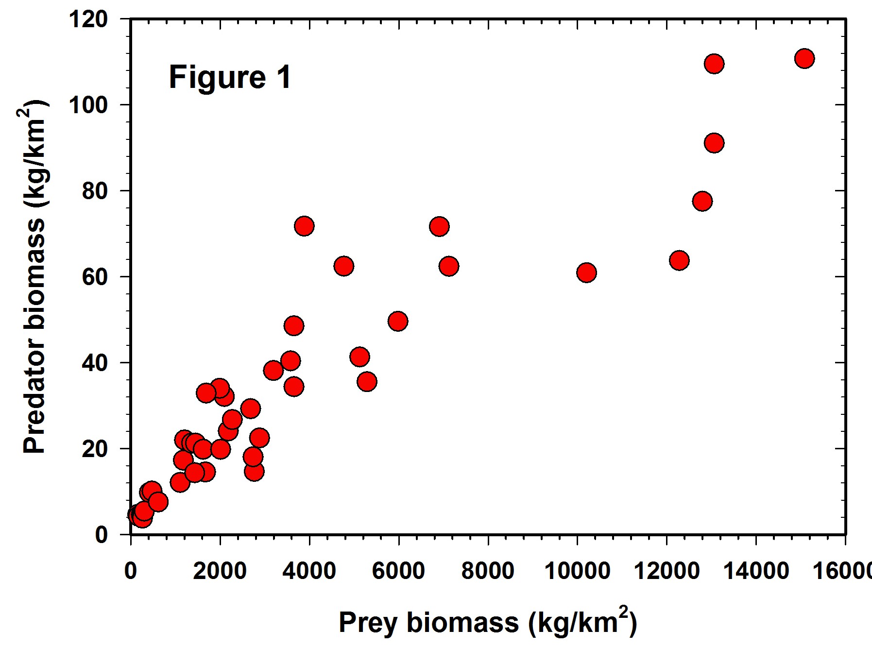
Figure 1 shows the raw data reported in the Hatton et al. (2015) paper but plotted in arithmetic space. It is clear that the variance increases with the mean and the data are highly variable, as well as slightly curvilinear, so a transformation is clearly desirable for statistical analysis. Unfortunately we are given no error bars on each of the point estimates, so it is not possible to plot confidence limits for each estimate.

We log both the axes and get Figure 2 which is identical to that plotted as Figure 1 in Hatton et al. (2015). Clearly the regression fit is better that that of Figure 1 and yet there is still considerable variation around the line of best fit.

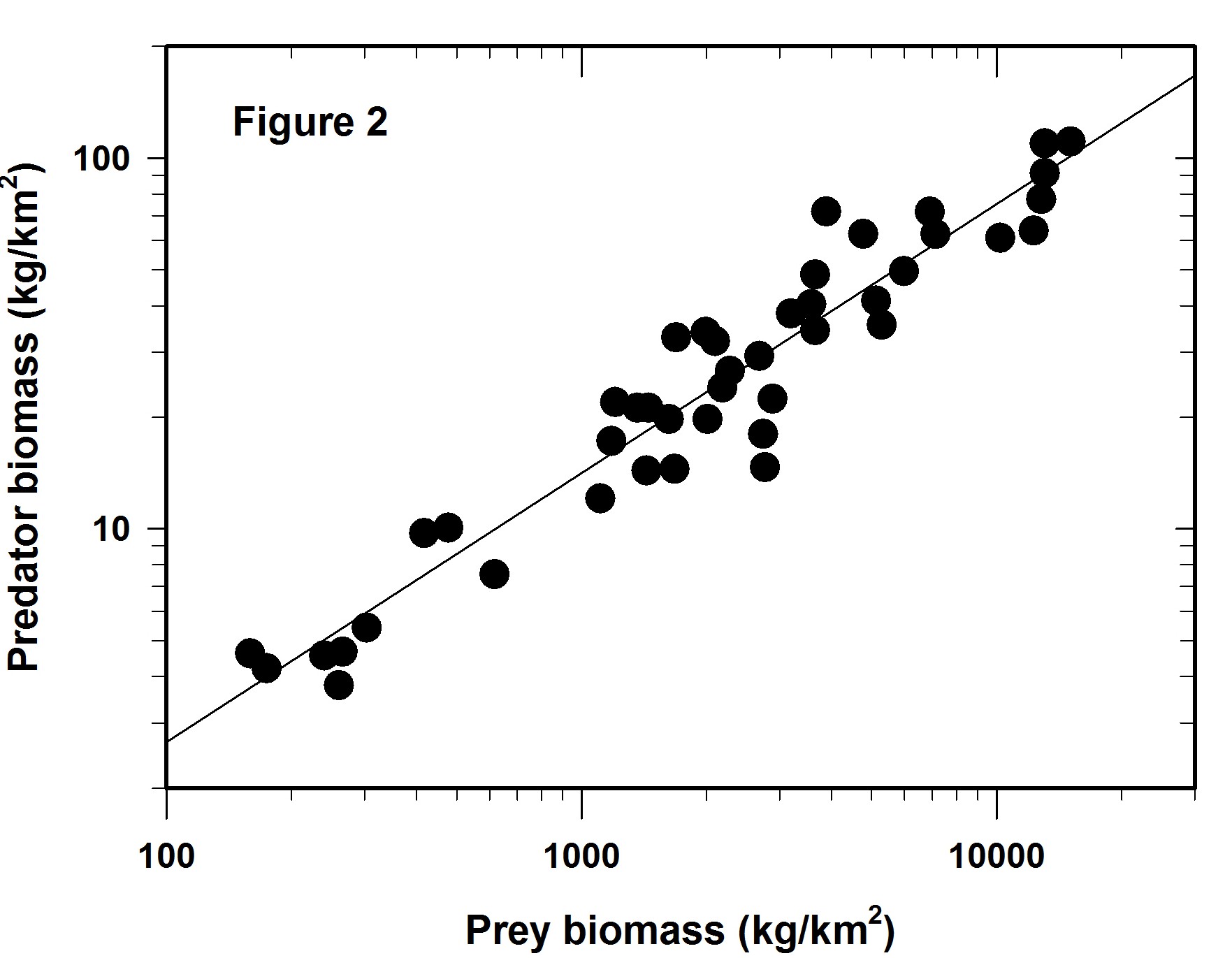
The variation around this log-log line is the main issue I wish to discuss here. Much depends on the reason for the regression line. Mac Nally (2000) made the point that regressions are often used for predictive purposes but sometimes used only as explanations. I assume here one wishes this to be a predictive regression.

So the next question is if the Figure 2 regression is predictive, how wide are the confidence limits? In this case we will adopt the usual 95% confidence predictions for a single data point. The result is shown in Figure 3, which did not appear in the Science article. The red lines define the 95% confidence belt.

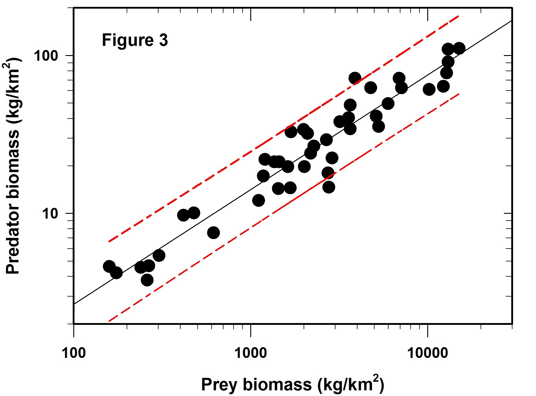
Now comes the main point of my concerns with log-log regressions. What do these error limits really mean when they are translated back to the original measurements that define the graph?

The table given below gives the prediction intervals for a hypothetical set of 8 prey abundances scattered along the span of prey densities reported.

The overall average confidence limits for this log-log regression are -43% to +75%, given that the SE of the predictions varies little across the range of values used in the regression. These are very broad confidence limits for any prediction from a regression line.

The bottom line is that log-log regressions can camouflage a great deal of variation, which may or may not be acceptable depending on the use of the regression. These plots always visually look much better than they are. You probably already knew this but I worry that it is a point that can be easily overlooked.

Lastly, a minor quibble with this regression. Some authors (e.g. Ricker 1983, Smith 2009) have discussed the issue of using the reduced major axis (or geometric mean regression) when the X variable is measured with error instead of the standard regression method. One could argue for this particular data set that the X variable is measured with error, so that I have used a reduced major axis regression in this discussion. The overall conclusions are not changed if standard regression methods are used.

Hatton, I.A., McCann, K.S., Fryxell, J.M., Davies, T.J., Smerlak, M., Sinclair, A.R.E. & Loreau, M. (2015) The predator-prey power law: Biomass scaling across terrestrial and aquatic biomes. Science 349 (6252). doi: 10.1126/science.aac6284

Mac Nally, R. (2000) Regression and model-building in conservation biology, biogeography and ecology: The distinction between – and reconciliation of – ‘predictive’ and ‘explanatory’ models. Biodiversity & Conservation, 9, 655-671. doi: 10.1023/A:1008985925162

Ricker, W.E. (1984) Computation and uses of central trend lines. Canadian Journal of Zoology 62 (10), 1897-1905.doi: 10.1139/z84-279

Smith, R.J. (2009) Use and misuse of the reduced major axis for line-fitting. American Journal of Physical Anthropology, 140, 476-486. doi: 10.1002/ajpa.21090