Probability Distributions

Consider an event or series of events with a variety of possible outcomes. We define a random variable that represents a particular outcome of these events.

Random variables are generally denoted by capital letters, eg X, Y, Z.

For instance, toss a coin twice and record the number of heads. The number of heads is a random variable and it may take on three values: X=0 (no heads), X=1 (one head), and X=2 (two heads).

First, we will consider random variables, as in this example, which have only a discrete set of possible outcomes (eg 0, 1, 2).

In many cases of interest, one can specify the probability distribution that a random variable will follow.

That is, one can give the probability that X takes on a particular value x, written as P(X=x), for all possible values of x.

E.g., for a fair coin tossed twice, P(X=0)=1/4, P(X=1)=1/2, P(X=2)=1/4.

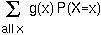
NOTE: Because X must take on some value, the sum of P(X=x) over all possible values of x must equal one:

Discrete Probability Distributions

Notice that you can find the expectation of a random variable from its distribution, you don't actually need to perform the experiment.

For example, E(number of heads in two coin tosses) = 0*P(X=0) + 1*P(X=1) + 2*P(X=2) = 0*1/4 + 1*1/2 + 2*1/4 = 1. You expect to see one head on average in two coin tosses.

Some useful facts about expectations:

• E(cX) = c E(X) if c is a constant

• E(X+Y) = E(X) + E(Y) "the expectation of a sum equals the sum of the expectations"

• E(XY) = E(X) E(Y) ONLY if X and Y are independent random variables.

• E[g(X)] =

Discrete Probability Distributions

Another common measure of dispersion is the standard deviation, SD(X), which equals the square root of Var(X).

But how do we calculate the variance?

Notice that E[(X-)²] = E[X² - 2X + ²]. We simplify this using the above rules.

First, because the expectation of a sum equals the sum of expectations: Var(X) = E[X²] - E[2X] + E[²].

Then, because constants may be taken out of an expectation: Var(X) = E[X²] - 2 E[X] + ² E[1] = E[X²] - 2 ² + ² = E[X²] - ².

Finally, notice that E[X²] can be written as E[g(X)] where g(X)=X². From the final fact about expectations, we can calculate this:

For example, for the coin toss, E[X²] = (0)²*P(X=0) + (1)²*P(X=1) + (2)²*P(X=2) = 0*1/4 + 1*1/2 + 4*1/4 = 3/2. From this we calculate the variance, Var(x) = E[X²] - ² = 3/2 - (1)² = 1/2.

Useful facts about variances:

• Var(cX) = c² Var(X) if c is a constant

• Var(X+Y) = Var(X) + Var(Y) ONLY if X and Y are independent.

Discrete Probability Distributions

It is worth knowing what type of distribution you expect under different circumstances, because if you expect a particular distribution you can determine the mean and variance that you expect to observe.

If n=1, the probability of getting a zero in the trial is P(X=0)=1-p. The probability of getting a one in the trial is P(X=1)=p. These are the only possibilities [P(X=0)+P(X=1)=1].

If n=2, the probability of getting two zeros is P(X=0) = (1-p)² (getting a zero on the first trial and then independently getting a zero on the second trial), the probability of getting a one is P(X=1) = p(1-p) + (1-p)p = 2 p (1-p), and the probability of getting two ones is P(X=2) = p². These are the only possibilities [P(X=0)+P(X=1)+P(X=2)=1].

For general n, we use the binomial distribution to determine the probability of k "ones" in n trials:

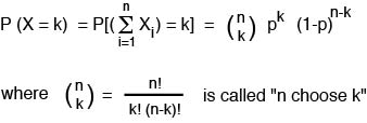
"n choose k" is the number of ways that you can arrange k ones and n-k zeros in a row. For instance, if you wrote down, in a row, the results of n coin tosses, the number of different ways that you could write down all the outcomes and have exactly k heads is "n choose k".

Discrete Probability Distributions

We can draw the probability distribution given specific values of p:

The mean of the binomial distribution equals E(X)=np.

Proof: The expectation of the sum of X_i equals the sum of the expected values of X_i, but E[X_i] equals p so the sum over n such trials equals np.

The variance of the binomial distribution is equal to Var(X)=np(1-p).

Proof: Because each trial is independent, the variance of the sum of X_i equals the sum of the variances of X_i. Because Var(X_i) equals

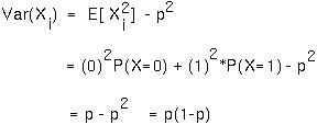
the sum of the variances will equal np(1-p).

Discrete Probability Distributions

The probability that the first "one" would appear on the first trial is p.

The probability that the first "one" appears on the second trial is (1-p)*p, because the first trial had to have been a zero followed by a one.

By generalizing this procedure, the probability that there will be k-1 failures before the first success is:

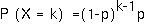
This is the geometric distribution.

A geometric distribution has a mean of 1/p and a variance of (1-p)/p².

Example: If the probability of extinction of an endangered population is estimated to be 0.1 every year, what is the expected time until extinction?

Notice though that the variance in this case is nearly 100! This means that the actual year in which the population will go extinct is very hard to predict accurately. We can see this from the distribution:

Discrete Probability Distributions

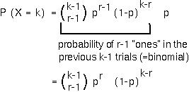
A negative binomial distribution has a mean = r/p and a variance = r(1-p)/p².

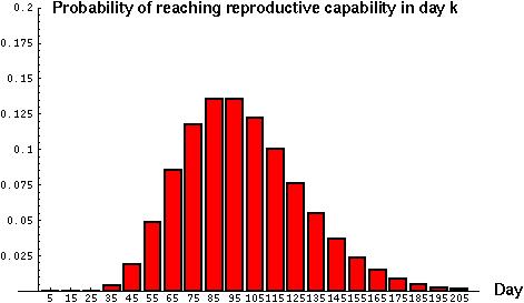
Example: If a predator must capture 10 prey before it can grow large enough to reproduce, what would the mean age of onset of reproduction be if the probability of capturing a prey on any given day is 0.1?

Notice that again the variance in this case is quite high (~1000) and that the distribution looks quite skewed (=not symmetric). Some predators will reach reproductive age much sooner and some much later than the average:

Discrete Probability Distributions

First, it is an approximation to the binomial distribution when n is large and p is small.

Secondly, the Poisson describes the number of events that will occur in a given time period when the events occur randomly and are independent of one another. Similarly, the Poisson distribution describes the number of events in a given area when the presence or absence of a point is independent of occurrences at other points.

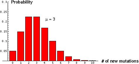
The Poisson distribution looks like:

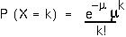
A Poisson distribution has the unique property that its variance equals its mean, . When the Poisson is used as an approximation to the binomial, the mean and the variance both equal np.

Discrete Probability Distributions

Example: If hummingbirds arrive at a flower at a rate per hour, how many visits are expected in x hours of observation and what is the variance in this expectation? If significantly more variance is observed than expected, what might this tell you about hummingbird visits?

Example: (From Romano) If bacteria are spread across a plate at an average density of 5000 per square inch, what is the chance of seeing no bacteria in the viewing field of a microscope if this viewing field is 10^-4 square inches? What, therefore, is the probability of seeing at least one cell?

Back to biology 301 home page.