plot of chunk unnamed-chunk-2
| make.musse.split {diversitree} | R Documentation |
Create a likelihood function for a MuSSE model where the tree is partitioned into regions with different parameters.
make.musse.split(tree, states, k, nodes, split.t,
                 sampling.f=NULL, strict=TRUE, control=list())
tree |
An ultrametric bifurcating phylogenetic tree, in
|
states |
A vector of character states, each of which must be an
integer between 1 and |
k |
The number of states. |
nodes |
Vector of nodes that will be split (see Details). |
split.t |
Vector of split times, same length as |
sampling.f |
Vector of length |
strict |
The |
control |
List of control parameters for the ODE solver. See
details in |
Branching times can be controlled with the split.t
argument. If this is Inf, split at the base of the branch (as in
MEDUSA). If 0, split at the top (closest to the present, as in
the new option for MEDUSA). If 0 < split.t < Inf then we split
at that time on the tree (zero is the present, with time growing
backwards).
Richard G. FitzJohn
This example picks up from the tree used in the ?make.musse example.
First, simulate the tree:
set.seed(2)
pars <- c(.1, .15, .2, # lambda 1, 2, 3
.03, .045, .06, # mu 1, 2, 3
.05, 0, # q12, q13
.05, .05, # q21, q23
0, .05) # q31, q32
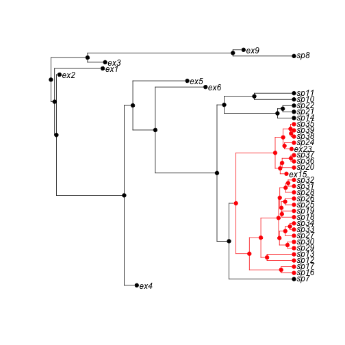
phy <- tree.musse(pars, 30, x0=1)Here is the phylogeny, with true character history superposed:
h <- history.from.sim.discrete(phy, 1:3)
plot(h, phy, show.node.label = TRUE, font = 1, cex = 0.75, no.margin = TRUE)
plot of chunk unnamed-chunk-2
Here is a plain MuSSE function for later comparison:
lik.m <- make.musse(phy, phy$tip.state, 3)
lik.m(pars)  # -110.8364
## [1] -110.8Split this phylogeny at three points: nd16 and nd25, splitting it into three chunks
nodes <- c("nd16", "nd25")
nodelabels(node = match(nodes, phy$node.label) + length(phy$tip.label),
    pch = 19, cex = 2, col = "#FF000099")
## Error: plot.new has not been called yetTo make a split BiSSE function, pass the node locations and times in. Here, we'll use 'Inf' as the split time to mimick MEDUSA's behaviour of placing the split at the base of the branch subtended by a node.
lik.s <- make.musse.split(phy, phy$tip.state, 3, nodes, split.t = Inf)The parameters must be a list of the same length as the number of partitions. Partition '1' is the root partition, and partition i is the partition rooted at the node[i-1]:
argnames(lik.s)## [1] "lambda1.1" "lambda2.1" "lambda3.1" "mu1.1" "mu2.1"
## [6] "mu3.1" "q12.1" "q13.1" "q21.1" "q23.1"
## [11] "q31.1" "q32.1" "lambda1.2" "lambda2.2" "lambda3.2"
## [16] "mu1.2" "mu2.2" "mu3.2" "q12.2" "q13.2"
## [21] "q21.2" "q23.2" "q31.2" "q32.2" "lambda1.3"
## [26] "lambda2.3" "lambda3.3" "mu1.3" "mu2.3" "mu3.3"
## [31] "q12.3" "q13.3" "q21.3" "q23.3" "q31.3"
## [36] "q32.3" Because we have two nodes, there are three sets of parameters. Replicate the original list to get a starting point for the analysis:
pars.s <- rep(pars, 3)
names(pars.s) <- argnames(lik.s)

lik.s(pars.s)  # -110.8364
## [1] -110.8This is basically identical (to acceptable tolerance) to the plain MuSSE version:
lik.s(pars.s) - lik.m(pars)## [1] 5.989e-08The resulting likelihood function can be used in ML analyses with find.mle. However, because of the large number of parameters, this may take some time (especially with as few species as there are in this tree - getting convergence in a reasonable number of iterations is difficult).
[This section is not run by default]
fit.s <- find.mle(lik.s, pars.s, control = list(maxit = 20000))[Ends not run section]
Bayesian analysis also works, using the mcmc function. Given the large number of parameters, priors will be essential, as there will be no signal for several parameters. Here, I am using an exponential distribution with a mean of twice the state-independent diversification rate.
[This section is not run by default]
prior <- make.prior.exponential(1/(-2 * diff(starting.point.bd(phy))))
samples <- mcmc(lik.s, pars.s, 100, prior = prior, w = 1, print.every = 10)
[Ends not run section]