R: Binary State Speciation and Extinction Model: Time Dependant...

make.bisse.td {diversitree}

R Documentation

Binary State Speciation and Extinction Model: Time Dependant Models

Description

Create a likelihood function for a BiSSE model where different chunks of time have different parameters. This code is experimental!

Usage

make.bisse.td(tree, states, n.epoch, unresolved=NULL, sampling.f=NULL,
              nt.extra=10, strict=TRUE, control=list())
make.bisse.t(tree, states, functions, unresolved=NULL, sampling.f=NULL,
             nt.extra=10, strict=TRUE, control=list())

Arguments

`tree`	An ultrametric bifurcating phylogenetic tree, in `ape` “phylo” format.
`states`	A vector of character states, each of which must be 0 or 1, or `NA` if the state is unknown. This vector must have names that correspond to the tip labels in the phylogenetic tree (`tree$tip.label`). For tips corresponding to unresolved clades, the state should be `NA`.
`n.epoch`	Number of epochs. 1 corresponds to plain BiSSE, so this will generally be an integer at least 2.
`functions`	A named list of functions of time. See details.
`unresolved`	Unresolved clade information: see `make.bisse`. (Currently this is not supported.)
`sampling.f`	Vector of length 2 with the estimated proportion of extant species in state 0 and 1 that are included in the phylogeny. See `make.bisse`.
`nt.extra`	The number of species modelled in unresolved clades (this is in addition to the largest observed clade).
`strict`	The `states` vector is always checked to make sure that the values are 0 and 1 only. If `strict` is `TRUE` (the default), then the additional check is made that every state is present. The likelihood models tend to be poorly behaved where states are missing.
`control`	List of control parameters for the ODE solver. See details in `make.bisse`.

Details

This builds a BiSSE likelihood function where different regions of time (epochs) have different parameter sets. By default, all parameters are free to vary between epochs, so some constraining will probably be required to get reasonable answers.

For n epochs, there are n-1 time points; the first n-1 elements of the likelihood's parameter vector are these points. These are measured from the present at time zero, with time increasing towards the base of the tree. The rest of the parameter vector are BiSSE parameters; the elements n:(n+6) are for the first epoch (closest to the present), elements (n+7):(n+13) are for the second epoch, and so on.

For make.bisse.t, the funtions is a list of functions of time. For example, to have speciation rates be linear functions of time, while the extinction and character change rates be constant with respect to time, one can do

functions=rep(list(linear.t, constant.t), c(2, 4))

The functions here must have t as their first argument, interpreted as time back from the present. See make.pars.t for more information, and for some potentially useful time functions.

Author(s)

Richard G. FitzJohn

Examples

set.seed(4)
pars <- c(0.1, 0.2, 0.03, 0.03, 0.01, 0.01)
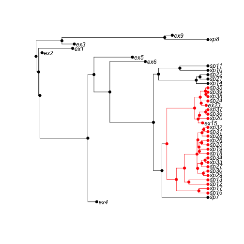
phy <- tree.bisse(pars, max.t = 30, x0 = 0)

Suppose we want to see if diversification is different in the most recent 3 time units, compared with the rest of the tree (yes, this is a totally contrived example!):

plot(phy)
axisPhylo()
abline(v = max(branching.times(phy)) - 3, col = "red", lty = 3)

plot of chunk unnamed-chunk-2

For comparison, make a plain BiSSE likelihood function

lik.b <- make.bisse(phy, phy$tip.state)

Create the time-dependent likelihood function. The final argument here is the number of 'epochs' that are allowed. Two epochs is one switch point.

lik.t <- make.bisse.td(phy, phy$tip.state, 2)

The switch point is the first argument. The remaining 12 parameters are the BiSSE parameters, with the first 6 being the most recent epoch.

argnames(lik.t)

##  [1] "t.1"       "lambda0.1" "lambda1.1" "mu0.1"     "mu1.1"    
##  [6] "q01.1"     "q10.1"     "lambda0.2" "lambda1.2" "mu0.2"    
## [11] "mu1.2"     "q01.2"     "q10.2"


pars.t <- c(3, pars, pars)
names(pars.t) <- argnames(lik.t)

Calculations are identical to a reasonable tolerance:

lik.b(pars) - lik.t(pars.t)

## [1] -8.144e-07

It will often be useful to constrain the time as a fixed quantity.

lik.t2 <- constrain(lik.t, t.1 ~ 3)

Parameter estimation under maximum likelihood. This is marked "don't run" because the time-dependent fit takes a few minutes.

[This section is not run by default] Fit the BiSSE ML model

fit.b <- find.mle(lik.b, pars)

And fit the BiSSE/td model

fit.t <- find.mle(lik.t2, pars.t[argnames(lik.t2)], control = list(maxit = 20000))

Compare these two fits with a likelihood ratio test (lik.t2 is nested within lik.b)

anova(fit.b, td = fit.t)

[Ends not run section]

The time varying model (bisse.t) is more general, but substantially slower. Here, I will show that the two functions are equivalent for step function models. We'll constrain all the non-lambda parameters to be the same over a time-switch at t=5. This leaves 8 parameters.

lik.td <- make.bisse.td(phy, phy$tip.state, 2)
lik.td2 <- constrain(lik.td, t.1 ~ 5, mu0.2 ~ mu0.1, mu1.2 ~ mu1.1, 
    q01.2 ~ q01.1, q10.2 ~ q10.1)

lik.t <- make.bisse.t(phy, phy$tip.state, rep(list(stepf.t, constant.t), 
    c(2, 4)))
lik.t2 <- constrain(lik.t, lambda0.tc ~ 5, lambda1.tc ~ 5)

Note that the argument names for these functions are different from one another. This reflects different ways that the functions will tend to be used, but is potentially confusing here.

argnames(lik.td2)

## [1] "lambda0.1" "lambda1.1" "mu0.1"     "mu1.1"     "q01.1"     "q10.1"    
## [7] "lambda0.2" "lambda1.2"

argnames(lik.t2)

## [1] "lambda0.y0" "lambda0.y1" "lambda1.y0" "lambda1.y1" "mu0"       
## [6] "mu1"        "q01"        "q10"

First, evaluate the functions with no time effect and check that they are the same as the base BiSSE model

p.td <- c(pars, pars[1:2])
p.t <- pars[c(1, 1, 2, 2, 3:6)]

All agree:

lik.b(pars)  # -159.7128

## [1] -159.7

lik.td2(p.td)  # -159.7128

## [1] -159.7

lik.t2(p.t)  # -159.7128

## [1] -159.7

In fact, the time-varying BiSSE will tend to be identical to plain BiSSE where the functions to not change:

lik.b(pars) - lik.t2(p.t)

## [1] 0

Slight numerical differences are typical for the time-chunk BiSSE, because it forces the integration to be carried out more carefully around the switch point.

lik.b(pars) - lik.td2(p.td)

## [1] -1.2e-06

Next, evaluate the functions with a time effect (5 time units ago, speciation rates were twice the contemporary rate)

p.td2 <- c(pars, pars[1:2] * 2)
p.t2 <- c(pars[1], pars[1] * 2, pars[2], pars[2] * 2, pars[3:6])

Huge drop in the likelihood (from -159.7128 to -172.7874)

lik.b(pars)

## [1] -159.7

lik.td2(p.td2)

## [1] -172.8

lik.t2(p.t2)

## [1] -172.8

The small difference remains between the two approaches, but they are basically the same.

lik.td2(p.td2) - lik.t2(p.t2)

## [1] 3.553e-06

There is a time cost to both time-dependent methods, but it is more heavily paid for the time-varying case:

system.time(lik.b(pars))

##    user  system elapsed 
##   0.007   0.000   0.007

system.time(lik.td2(p.td))  # 1.9x slower than plain BiSSE

##    user  system elapsed 
##   0.013   0.000   0.013

system.time(lik.t2(p.t))  # 10x  slower than plain BiSSE

##    user  system elapsed 
##   0.093   0.002   0.096

[Package diversitree version 0.9-4 ]