R: Binary State Speciation and Extinction Model

make.bisse {diversitree}

R Documentation

Binary State Speciation and Extinction Model

Description

Prepare to run BiSSE (Binary State Speciation and Extinction) on a phylogenetic tree and character distribution. This function creates a likelihood function that can be used in maximum likelihood or Bayesian inference.

Usage

make.bisse(tree, states, unresolved=NULL, sampling.f=NULL, nt.extra=10,
           strict=TRUE, control=list())
starting.point.bisse(tree, q.div=5, yule=FALSE)

Arguments

`tree`	An ultrametric bifurcating phylogenetic tree, in `ape` “phylo” format.
`states`	A vector of character states, each of which must be 0 or 1, or `NA` if the state is unknown. This vector must have names that correspond to the tip labels in the phylogenetic tree (`tree$tip.label`). For tips corresponding to unresolved clades, the state should be `NA`.
`unresolved`	Unresolved clade information: see section below for structure.
`sampling.f`	Vector of length 2 with the estimated proportion of extant species in state 0 and 1 that are included in the phylogeny. A value of `c(0.5, 0.75)` means that half of species in state 0 and three quarters of species in state 1 are included in the phylogeny. By default all species are assumed to be known.
`nt.extra`	The number of species modelled in unresolved clades (this is in addition to the largest observed clade).
`control`	List of control parameters for the ODE solver. See details below.
`strict`	The `states` vector is always checked to make sure that the values are 0 and 1 only. If `strict` is `TRUE` (the default), then the additional check is made that every state is present. The likelihood models tend to be poorly behaved where states are missing.
`q.div`	Ratio of diversification rate to character change rate. Eventually this will be changed to allow for Mk2 to be used for estimating q parameters.
`yule`	Logical: should starting parameters be Yule estimates rather than birth-death estimates?

Details

make.bisse returns a function of class bisse. This function has argument list (and default values)

    f(pars, condition.surv=TRUE, root=ROOT.OBS, root.p=NULL,
      intermediates=FALSE)

The arguments are interpreted as

pars A vector of six parameters, in the order lambda0, lambda1, mu0, mu1, q01, q10.
condition.surv (logical): should the likelihood calculation condition on survival of two lineages and the speciation event subtending them? This is done by default, following Nee et al. 1994.
root: Behaviour at the root (see Maddison et al. 2007, FitzJohn et al. 2009). The possible options are
- ROOT.FLAT: A flat prior, weighting D0 and D1 equally.
- ROOT.EQUI: Use the equilibrium distribution of the model, as described in Maddison et al. (2007).
- ROOT.OBS: Weight D0 and D1 by their relative probability of observing the data, following FitzJohn et al. 2009:
  
  D = D0 * D0/(D0 + D1) + D1 * D1/(D0 + D1)
- ROOT.GIVEN: Root will be in state 0 with probability root.p[1], and in state 1 with probability root.p[2].
- ROOT.BOTH: Don't do anything at the root, and return both values. (Note that this will not give you a likelihood!).
root.p: Root weightings for use when root=ROOT.GIVEN. sum(root.p) should equal 1.
intermediates: Add intermediates to the returned value as attributes:
- cache: Cached tree traversal information.
- intermediates: Mostly branch end information.
- vals: Root D values.
At this point, you will have to poke about in the source for more information on these.

starting.point.bisse produces a heuristic starting point to start from, based on the character-independent birth-death model. You can probably do better than this; see the vignette, for example. bisse.starting.point is the same code, but deprecated in favour of starting.point.bisse - it will be removed in a future version.

Unresolved clade information

This must be a data.frame with at least the four columns

tip.label, giving the name of the tip to which the data applies
Nc, giving the number of species in the clade
n0, n1, giving the number of species known to be in state 0 and 1, respectively.

These columns may be in any order, and additional columns will be ignored. (Note that column names are case sensitive).

An alternative way of specifying unresolved clade information is to use the function make.clade.tree to construct a tree where tips that represent clades contain information about which species are contained within the clades. With a clade.tree, the unresolved object will be automatically constructed from the state information in states. (In this case, states must contain state information for the species contained within the unresolved clades.)

ODE solver control

The differential equations that define the BiSSE model are solved numerically using deSolve's LSODA ODE solver or the CVODES solver from the SUNDIALS suite of solvers. The control argument to make.bisse controls the behaviour of the integrator. This is a list that may contain elements:

tol: Numerical tolerance used for the calculations. The default value of 1e-8 should be a reasonable trade-off between speed and accuracy. Do not expect too much more than this from the abilities of most machines!
eps: A value that when the sum of the D values drops below, the integration results will be discarded and the integration will be attempted again (the second-chance integration will divide a branch in two and try again, recursively until the desired accuracy is reached). The default value of 0 will only discard integration results when the parameters go negative. However, for some problems more restrictive values (on the order of control$tol) will give better stability.
backend: Select the solver. The three options here are
- deSolve: (the default for now). Use the LSODA solver from the deSolve package.
- cvodes: Use the CVODES solver from the SUNDIALS suite.
- CVODES: Use the CVODES solver, but also use an experimental, faster, function for the tree traversal.
safe(logical) Use a safer, slower, integrator when using the deSolve integrator? Leave this alone (this will be automatically selected when appropriate).

deSolve is the only supported backend on Windows.

Author(s)

Richard G. FitzJohn

References

FitzJohn R.G., Maddison W.P., and Otto S.P. 2009. Estimating trait-dependent speciation and extinction rates from incompletely resolved phylogenies. Syst. Biol. 58:595-611.

Maddison W.P., Midford P.E., and Otto S.P. 2007. Estimating a binary character's effect on speciation and extinction. Syst. Biol. 56:701-710.

Nee S., May R.M., and Harvey P.H. 1994. The reconstructed evolutionary process. Philos. Trans. R. Soc. Lond. B Biol. Sci. 344:305-311.

Examples

pars <- c(0.1, 0.2, 0.03, 0.03, 0.01, 0.01)
set.seed(4)
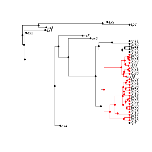
phy <- tree.bisse(pars, max.t = 30, x0 = 0)

Here is the 52 species tree with the true character history coded. Red is state '1', which has twice the speciation rate of black (state '0').

h <- history.from.sim.discrete(phy, 0:1)
plot(h, phy)

plot of chunk unnamed-chunk-2


lik <- make.bisse(phy, phy$tip.state)
lik(pars)  # -159.71

## [1] -159.7

Heuristic guess at a starting point, based on the constant-rate birth-death model (uses make.bd).

p <- starting.point.bisse(phy)

Start an ML search from this point. This takes some time (~7s)

fit <- find.mle(lik, p, method = "subplex")
logLik(fit)  # -158.6875

## 'log Lik.' -158.7 (df=6)

The estimated parameters aren't too far away from the real ones, even with such a small tree

rbind(real = pars, estimated = round(coef(fit), 2))

##           lambda0 lambda1  mu0  mu1  q01  q10
## real         0.10    0.20 0.03 0.03 0.01 0.01
## estimated    0.14    0.18 0.12 0.04 0.00 0.02

Test a constrained model where the speciation rates are set equal (takes ~4s).

lik.l <- constrain(lik, lambda1 ~ lambda0)
fit.l <- find.mle(lik.l, p[-1], method = "subplex")
logLik(fit.l)  # -158.7357

## 'log Lik.' -158.7 (df=5)

Despite the difference in the estimated parameters, there is no statistical support for this difference:

anova(fit, equal.lambda = fit.l)

##              Df lnLik AIC  ChiSq Pr(>|Chi|)
## full          6  -159 329                  
## equal.lambda  5  -159 327 0.0965       0.76

Run an MCMC. Because we are fitting six parameters to a tree with only 50 species, priors will be needed. I will use an exponential prior with rate 1/(2r), where r is the character independent diversificiation rate:

prior <- make.prior.exponential(1/(2 * (p[1] - p[3])))

This takes quite a while to run, so is not run by default

[This section is not run by default]

tmp <- mcmc(lik, fit$par, nsteps = 100, prior = prior, w = 0.1, print.every = 0)

w <- diff(sapply(tmp[2:7], range))
samples <- mcmc(lik, fit$par, nsteps = 1000, prior = prior, w = w, 
    print.every = 100)

See profiles.plot for more information on plotting these profiles.

col <- c("blue", "red")
profiles.plot(samples[c("lambda0", "lambda1")], col.line = col, las = 1, 
    xlab = "Speciation rate", legend = "topright")

[Ends not run section]

BiSSE reduces to the birth-death model and Mk2 when diversification is state independent (i.e., lambda0 ~ lambda1 and mu0 ~ mu1).

lik.mk2 <- make.mk2(phy, phy$tip.state)
lik.bd <- make.bd(phy)

BiSSE / Birth-Death Set the q01 and q10 parameters to arbitrary numbers (need not be symmetric), and constrain the lambdas and mus to be the same for each state. The likelihood function now has just two parameters and will be proprtional to Nee's birth-death based likelihood:

lik.bisse.bd <- constrain(lik, lambda1 ~ lambda0, mu1 ~ mu0, q01 ~ 
    0.01, q10 ~ 0.02)
pars <- c(0.1, 0.03)

These differ by -167.3861 for both parameter sets:

lik.bisse.bd(pars) - lik.bd(pars)

## [1] -167.4

lik.bisse.bd(2 * pars) - lik.bd(2 * pars)

## [1] -167.4

BiSSE / Mk2 Same idea as above: set all diversification parameters to arbitrary values (but symmetric this time):

lik.bisse.mk2 <- constrain(lik, lambda0 ~ 0.1, lambda1 ~ 0.1, mu0 ~ 
    0.03, mu1 ~ 0.03)

Differ by -150.4740 for both parameter sets.

lik.bisse.mk2(pars) - lik.mk2(pars)

## [1] -150.5

lik.bisse.mk2(2 * pars) - lik.mk2(2 * pars)

## [1] -150.5

Sampled BiSSE / Birth-Death Pretend that the tree is only .6 sampled:

lik.bd2 <- make.bd(phy, sampling.f = 0.6)
lik.bisse2 <- make.bisse(phy, phy$tip.state, sampling.f = c(0.6, 
    0.6))
lik.bisse2.bd <- constrain(lik.bisse2, lambda1 ~ lambda0, mu1 ~ mu0, 
    q01 ~ 0.01, q10 ~ 0.01)

Difference of -167.2876

lik.bisse2.bd(pars) - lik.bd2(pars)

## [1] -167.3

lik.bisse2.bd(2 * pars) - lik.bd2(2 * pars)

## [1] -167.3

Unresolved clade BiSSE / Birth-Death

set.seed(1)
unresolved <- data.frame(tip.label = I(sample(phy$tip.label, 5)), 
    Nc = sample(2:10, 5), n0 = 0, n1 = 0)
unresolved.bd <- structure(unresolved$Nc, names = unresolved$tip.label)
lik.bisse3 <- make.bisse(phy, phy$tip.state, unresolved)
lik.bisse3.bd <- constrain(lik.bisse3, lambda1 ~ lambda0, mu1 ~ mu0, 
    q01 ~ 0.01, q10 ~ 0.01)
lik.bd3 <- make.bd(phy, unresolved = unresolved.bd)

Difference of -167.1523

lik.bisse3.bd(pars) - lik.bd3(pars)

## [1] -167.2

lik.bisse3.bd(pars * 2) - lik.bd3(pars * 2)

## [1] -167.2

[This section is not run by default] This only works when diversitree was built with CVODES support (currently not on Windows). This support is still experimental.

Different backends:

lik.1 <- make.bisse(phy, phy$tip.state, control = list(backend = "deSolve"))
lik.2 <- make.bisse(phy, phy$tip.state, control = list(backend = "cvodes"))
lik.3 <- make.bisse(phy, phy$tip.state, control = list(backend = "CVODES"))

All the calculations are very similar

pars <- c(0.1, 0.2, 0.03, 0.03, 0.01, 0.01)
(ll.1 <- lik.1(pars))
(ll.2 <- lik.2(pars))
(ll.3 <- lik.3(pars))
diff(range(c(ll.1, ll.2, ll.3)))

However, the CVODES version is quite a bit faster than the other two (cvodes is often a bit slower than deSolve).

Timings are on a 2008 Mac Pro

system.time(fit.1 <- find.mle(lik.1, pars))  # 4.5s
system.time(fit.2 <- find.mle(lik.2, pars))  # 6.0s
system.time(fit.3 <- find.mle(lik.3, pars))  # 1.6s

All found the same ML point:

diff(range(fit.1$lnLik, fit.2$lnLik, fit.3$lnLik))