Ancestral State Reconstruction Under Mk2/Mkn

Description

Perform ancestral state reconstruction under Mk2 and other constant rate Markov models. Marginal, joint, and stochastic reconstructions are supported. Documentation is still in an early stage, and mostly in terms of examples.

Usage

## S3 method for class 'mkn'
make.asr.marginal(lik, ...)
## S3 method for class 'mkn'
make.asr.joint(lik, ...)
## S3 method for class 'mkn'
make.asr.stoch(lik, slim=FALSE, ...)

Arguments

Details

Output will differ slightly when mk2 and mkn models are used as lik, as mk2 uses states 0/1, while 2-state mkn uses 1/2.

This is all quite slow. Faster versions are coming eventually.

These functions all return functions that generate different types of ancestral reconstruction.

Author(s)

Richard G. FitzJohn

Examples

Start with a simple tree evolved under a constant rates birth-death model with asymetric character evolution

pars <- c(0.1, 0.1, 0.03, 0.03, 0.03, 0.06)
set.seed(1)
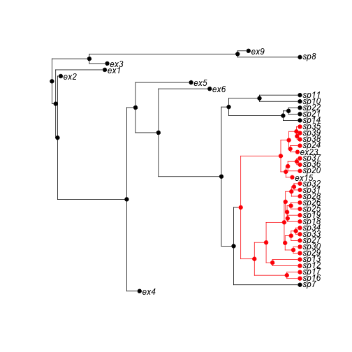
phy <- trees(pars, "bisse", max.taxa = 50, max.t = Inf, x0 = 0)[[1]]

Here is the true history. The root node appears to be state 1 (red) at the root, despite specifying a root of state 0 (x0=0, in statement above). This is because the tree started with a single lineage, but had changed state by the time the first speciation event happened.

h <- history.from.sim.discrete(phy, 0:1)
plot(h, phy, main = "True history")

plot of chunk unnamed-chunk-2

All of the methods need a likelihood function; build a mk2 function:

lik <- make.mk2(phy, phy$tip.state)

Using the true parameters, compute the marginal ancestral state reconstructions:

st.m <- asr.marginal(lik, pars[5:6])

There is still not a good stand-alone plotting command for nodes. For now, use ape's nodelabels().

plot(h, phy, main = "Marginal ASR", show.node.state = FALSE)
nodelabels(thermo = t(st.m), piecol = 1:2, cex = 0.5)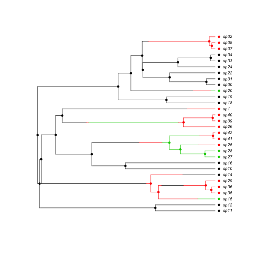

plot of chunk unnamed-chunk-5

Again, with the true parameters, a sample from the joint distribution:

st.j <- asr.joint(lik, pars[5:6])

Plotting this sample against the true values.

plot(h, phy, main = "Joint ASR", show.node.state = FALSE)
nodelabels(pch = 19, col = st.j + 1)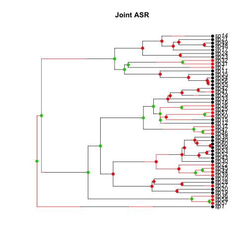

plot of chunk unnamed-chunk-7

This is just one sample, and is not very accurate in this case! Make 1,000 such samples and average them:

st.j2 <- asr.joint(lik, pars[5:6], 1000)
st.j2.mean <- colMeans(st.j2)

plot(h, phy, main = "Joint ASR (averaged)", show.node.state = FALSE)
nodelabels(thermo = 1 - st.j2.mean, piecol = 1:2, cex = 0.5)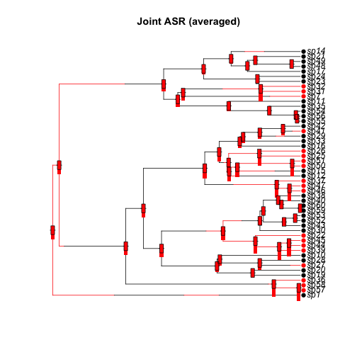

plot of chunk unnamed-chunk-8

Check the estimates against one another:

plot(st.m[2, ], st.j2.mean, xlab = "Marginal", ylab = "Joint", las = 1)
abline(0, 1)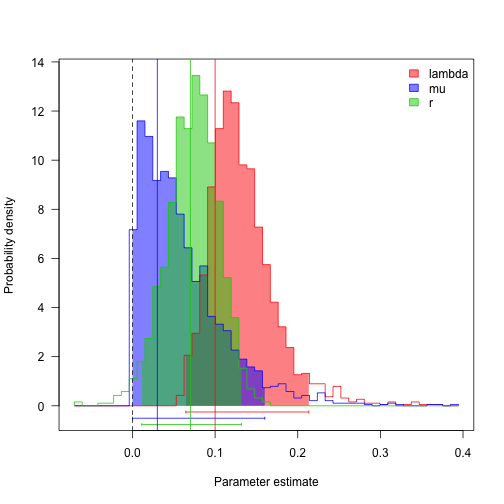

plot of chunk unnamed-chunk-9

Finally, the stochastic character mapping. This uses samples from the joint distribution at its core.

st.s <- asr.stoch(lik, pars[5:6])
plot(st.s, phy)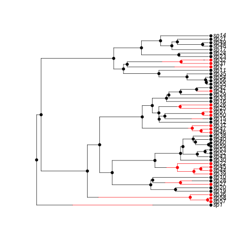

plot of chunk unnamed-chunk-10

Again, multiple samples can be done at once. There is a function for summarising histories, but it is still in the works.

Repeating the above with a two-state mkn model:

lik2 <- make.mkn(phy, phy$tip.state + 1, 2, FALSE)

Everything works:

st2.m <- asr.marginal(lik2, pars[5:6])
st2.j <- asr.joint(lik2, pars[5:6], 100)
st2.s <- asr.stoch(lik2, pars[5:6])

Marginal likelihoods agree:

all.equal(st.m, st2.m)

## [1] TRUE

Joint reconstructions are stochastic, so just check with a regression:

summary(lm(colMeans(st2.j) - 1 ~ colMeans(st.j2) - 1))

## 
## Call:
## lm(formula = colMeans(st2.j) - 1 ~ colMeans(st.j2) - 1)
## 
## Residuals:
##    Min     1Q Median     3Q    Max 
## -0.337 -0.319 -0.118  0.136  0.341 
## 
## Coefficients:
##                 Estimate Std. Error t value Pr(>|t|)    
## colMeans(st.j2)   0.3313     0.0255      13   <2e-16 ***
## ---
## Signif. codes:  0 '***' 0.001 '**' 0.01 '*' 0.05 '.' 0.1 ' ' 1 
## 
## Residual standard error: 0.258 on 48 degrees of freedom
## Multiple R-squared: 0.778,   Adjusted R-squared: 0.773 
## F-statistic:  168 on 1 and 48 DF,  p-value: <2e-16 
## 

Integrate parameter uncertainty, and see how far down the tree there is any real information on parameter states for this tree (this takes about 6s)

[This section is not run by default]

set.seed(1)
prior <- make.prior.exponential(0.5)
samples <- mcmc(lik, pars[5:6], 1000, w = 1, prior = prior, print.every = 100)
st.m.avg <- rowMeans(apply(samples[2:3], 1, asr.joint, lik = lik))

plot(h, phy, main = "MCMC Averaged ASR", show.node.state = FALSE)
nodelabels(thermo = 1 - st.m.avg, piecol = 1:2, cex = 0.5)

[Ends not run section]