Ancestral State Reconstruction Under BiSSE

Description

Perform ancestral state reconstruction under BiSSE and other constant rate Markov models. Marginal reconstructions are supported (c.f. asr). Documentation is still in an early stage, and mostly in terms of examples.

Usage

## S3 method for class 'bisse'
make.asr.marginal(lik, ...)
## S3 method for class 'musse'
make.asr.marginal(lik, ...)

Arguments

Author(s)

Richard G. FitzJohn

Examples

Start with a simple tree evolved under a BiSSE with all rates asymmetric:

pars <- c(0.1, 0.2, 0.03, 0.06, 0.01, 0.02)
set.seed(3)
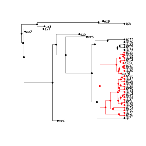
phy <- trees(pars, "bisse", max.taxa = 50, max.t = Inf, x0 = 0)[[1]]

Here is the true history

h <- history.from.sim.discrete(phy, 0:1)
plot(h, phy, main = "True history")

plot of chunk unnamed-chunk-2

BiSSE ancestral state reconstructions under the ML model

lik <- make.bisse(phy, phy$tip.state)
fit <- find.mle(lik, pars, method = "subplex")
st <- asr.marginal(lik, coef(fit))
nodelabels(thermo = t(st), piecol = 1:2, cex = 0.5)

## Error: plot.new has not been called yet

Mk2 ancestral state reconstructions, ignoring the shifts in diversification rates:

lik.m <- make.mk2(phy, phy$tip.state)
fit.m <- find.mle(lik.m, pars[5:6], method = "subplex")
st.m <- asr.marginal(lik.m, coef(fit.m))

The Mk2 results have more uncertainty at the root, but both are similar.

nodelabels(thermo = t(st.m), piecol = 1:2, cex = 0.5, adj = -0.5)

## Error: plot.new has not been called yet

[This section is not run by default] (This section will take 10 or so minutes to run.) Try integrating over parameter uncertainty and comparing the BiSSE with Mk2 output:

prior <- make.prior.exponential(2)
samples <- mcmc(lik, coef(fit), 1000, w = 1, prior = prior, print.every = 100)
st.b <- apply(samples[2:7], 1, function(x) asr.marginal(lik, x)[2, 
    ])
st.b.avg <- rowMeans(st.b)

samples.m <- mcmc(lik.m, coef(fit.m), 1000, w = 1, prior = prior, 
    print.every = 100)
st.m <- apply(samples.m[2:3], 1, function(x) asr.marginal(lik.m, 
    x)[2, ])
st.m.avg <- rowMeans(st.m)

These end up being more striking in their similarity than their differences, except for the root node, where BiSSE remains more sure that is in state 0 (there is about 0.05 red there).

plot(h, phy, main = "Marginal ASR, BiSSE (left), Mk2 (right)", show.node.state = FALSE)
nodelabels(thermo = 1 - st.b.avg, piecol = 1:2, cex = 0.5)
nodelabels(thermo = 1 - st.m.avg, piecol = 1:2, cex = 0.5, adj = -0.5)

[Ends not run section]

Equivalency of Mk2 and BiSSE where diversification is state independent. For any values of lambda/mu (here .1 and .03) where these do not vary across character states, these two methods will give essentially identical marginal ancestral state reconstructions.

st.id <- asr.marginal(lik, c(0.1, 0.1, 0.03, 0.03, coef(fit.m)))
st.id.m <- asr.marginal(lik.m, coef(fit.m))

Reconstructions are identical to a relative tolerance of 1e-7 (0.0000001), which is similar to the expected tolerance of the BiSSE calculations.

all.equal(st.id, st.id.m, tolerance = 1e-07)

## [1] TRUE

Equivalency of BiSSE and MuSSE reconstructions for two states:

lik.b <- make.bisse(phy, phy$tip.state)
lik.m <- make.musse(phy, phy$tip.state + 1, 2)

st.b <- asr.marginal(lik.b, coef(fit))
st.m <- asr.marginal(lik.m, coef(fit))

all.equal(st.b, st.m)

## [1] TRUE