Methods of Analysis. III. Stability

What happens to a point very near an equilibrium?

If points near an equilibrium tend to move towards the equilibrium over time, the equilibrium is said to be locally stable.

If points near an equilibrium tend to move away from the equilibrium over time, the equilibrium is said to be locally unstable.

By definition, when we say that an equilibrium point is locally stable, we mean that all solutions which begin from an initial condition close to converge to as time goes to infinity.

                                          -- Roughgarden p.557

An equilibrium point is said to be globally stable if all initial starting conditions lead to it.

Goal: To determine whether a small perturbation away from an equilibrium point will grow or shrink in magnitude over time.

Methods of Analysis. III. Stability

Mathematical Aside: Taylor Series

Most nicely behaved functions, f(x), can be rewritten as:

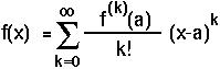
where is the kth derivative of the function with respect to x evaluated at the point a. (This is proven in many calculus books.)

How does this help?

If we have an equilibrium point, call it a, and we have a starting condition x which is near a, then we can use the Taylor Series to rewrite the equations that describe how the system changes over time.

If we start near enough to the equilibrium, (x-a)^k will be tiny for k greater than one and the function will be dominated by the first two terms in the sum with k=0 and k=1:

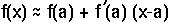
This is great! No matter how complicated and non-linear an equation we have, we can get an approximate equation that describes the dynamics near an equilibrium point. This approximate equation is linear in x and can be easily analysed.

Stability analysis in discrete one-variable models

Given a recursion equation in one variable (x[t+1] = f(x)) with an equilibrium , when will a small perturbation () away from the equilibrium grow in magnitude over time?

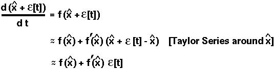
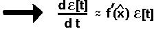
At time t, say that the population is a small distance from the equilibrium: + [t]. (Note that [t] might be negative.)

At time t+1, the population will be at + [t+1], which equals f( + [t]).

Using the Taylor Series of this function:

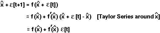
But we know that f() = , since at equilibrium the system does not change over time.

Therefore

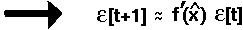
The perturbation will

• stay on the same side of the equilibrium if f'() is positive
  • and grow if f'() is greater than one ( locally unstable)
  • and shrink if f'() is between zero and one ( locally stable)

• move from one side of the equilibrium to the other side of the equilibrium if f'() is negative
  • and grow if f'() is below negative one ( locally unstable)
  • and shrink if f'() is between negative one and zero ( locally stable)

These conditions have a fairly simple graphical interpretation.

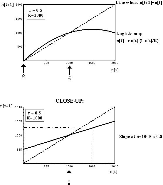
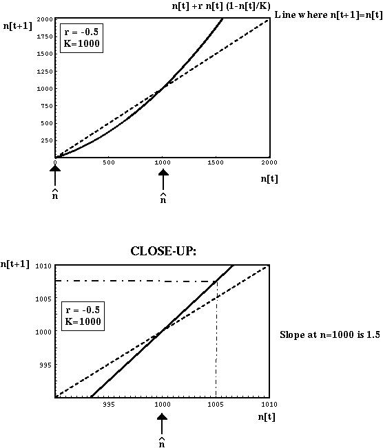
As an example, we'll consider the logistic equation in discrete time, with K=1000 and r=+/-0.5.

For populations started near carrying capacity (e.g. n[t]=1005), the slope of the recursion equation predicts whether the system will move closer to or further away from the equilibrium.

Stability analysis in continuous one-variable models

Again we focus on a small perturbation () away from an equilibrium () and determine whether this perturbation will grow or shrink.

If at time t the population is a small distance from equilibrium: + [t], the rate of change in x will be dx/dt = d( + [t])/dt.

In this case, dx/dt is the function that we wish to approximate using the Taylor Series:

Now, f() equals zero, since dx/dt = 0 at equilibrium.

Furthermore, by the linearity property of derivatives:

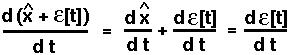
Therefore, the perturbation will change over time at a rate

The perturbation will

• grow if f'() is positive ( locally unstable),
• shrink if f'() is negative ( locally stable).

Exponential Growth Model

Let f(n) = n[t+1] = R n[t] and note that the only equilibrium is = 0.

For the stability analysis in discrete time we must find f'().

f'() therefore equals R.

• If R < 1, a perturbation near will shrink (=0 is locally stable).
• If R > 1, a perturbation near will grow (=0 is locally unstable).

Now let f(n) = dn/dt = r n. Again the only equilibrium is = 0.

For the stability analysis in continuouus time we must find f'().

f'() therefore equals r.

• If r < 0, a perturbation near will shrink (=0 is locally stable).
• If r > 0, a perturbation near will grow (=0 is locally unstable).

Haploid Selection Model (Discrete)

For the one-locus selection model, the recursion function is:

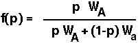
To perform a Taylor Series analysis, we first must find the derivative of f with respect to p:

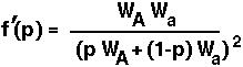
The first equilibrium of the haploid model is =0. At this equilibrium,

Therefore, if we start at some point near 0, say [t], then in the next generation the allele frequency will be approximately [t] W_A/W_a.

The allele frequency will move towards zero if W_A < W_a (=0 is locally stable).

The allele frequency will move away from zero if W_A > W_a (=0 is locally unstable).

Haploid Selection Model (Discrete)

The other equilibrium in the haploid model is =1. The derivative of the recursion function at this equilibrium is:

Therefore, if we start at some point near 1, say 1-[t], then in the next generation the allele frequency will be approximately 1-[t] W_a/W_A.

The allele frequency will move towards one if W_A > W_a (=1 is locally stable).

The allele frequency will move away from one if W_A < W_a (=1 is locally unstable).

Haploid Selection Model (Continuous)

A similar analysis can be performed using the continuous model. Now our function is dp/dt:

What will f'(p) equal?

There are two equilibria in this model, =0 and =1.

What will f'(0) equal?

When will =0 be stable?

When will =0 be unstable?

What will f'(1) equal?

When will =1 be stable?

When will =1 be unstable?

When A is favored, the population moves toward fixation on A and away from fixation on a (and vice versa).

Diploid Selection Model (Discrete)

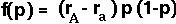
We have to evaluate f'() for each of the three equilibria of the diploid model, using the function, f(p), given by the recursion equation for the diploid selection model:

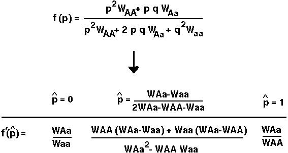
Results:

• Perturbations near =0 grow if W_Aa > W_aa but shrink if W_Aa < W_aa.
• Perturbation near =1 grow if W_Aa > W_AA but shrink if W_Aa < W_AA.

How Mathematica Can Make Life Easier

Diploid Selection Model (Discrete)

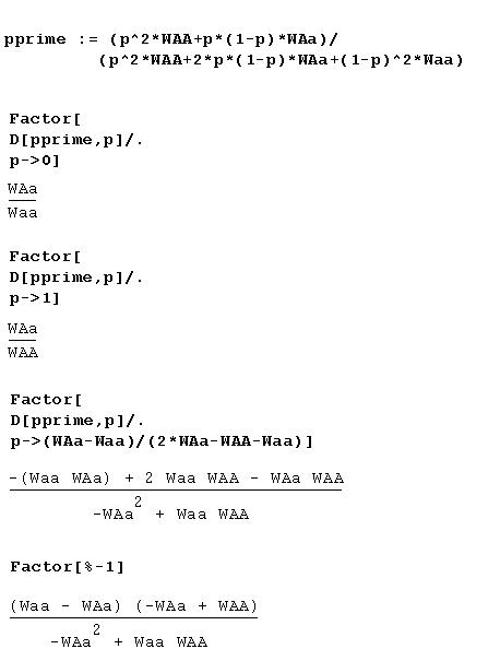
We can rewrite f'() as

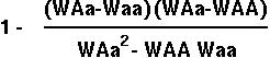
We need only look at the cases where the polymorphic equilibrium is valid (lies between 0 and 1):

• If W_AA < W_Aa > W_aa, a perturbation near will shrink (the internal polymorphic state is locally stable).
• If W_AA > W_Aa < W_aa, a perturbation near will grow (the internal polymorphic state is locally unstable).

• W_AA > W_Aa > W_aa (Directional selection favoring A)
  • Fixation on A is locally stable
  • Fixation on a is locally unstable
  • Polymorphic equilibrium is not valid.
• W_AA < W_Aa < W_aa (Directional selection favoring a)
  • Fixation on A is locally unstable
  • Fixation on a is locally stable
  • Polymorphic equilibrium is not valid.
• W_AA < W_Aa > W_aa (Heterozygote advantage or overdominance)
  • Fixation on A is locally unstable
  • Fixation on a is locally unstable
  • Polymorphic equilibrium is locally stable.
• W_AA > W_Aa < W_aa (Heterozygote disadvantage or underdominance)
  • Fixation on A is locally stable
  • Fixation on a is locally stable
  • Polymorphic equilibrium is locally unstable.

Back to biology 301 home page.