
Methods of Analysis. I. Graphs
Being able to "see" the results of a model is particularly important.
Often, the best first step in analysing a model is to graph the equations.
Today we will look at graphs that illustrate the behavior exhibited by the equations that we have developed.
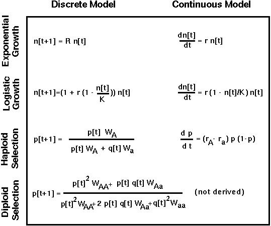
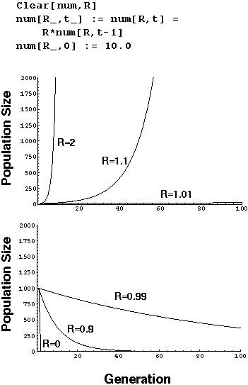
Exponential Growth Model (Discrete)
In this model, there is one parameter (R) which is the average number of offspring per parent:
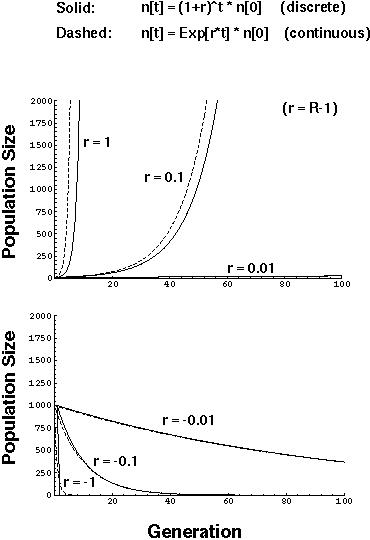
Exponential Growth Model (Discrete vs. Continuous)
Alternatively, if we define r as the growth rate (= R-1) then we can directly compare the discrete model (where growth is compounded per generation) and continuous model (where growth is compounded continuously):
Logistic Growth Model (Discrete)
In this model, there are two parameters (K,r). The behavior doesn't change much with different values of K (we'll use K=1000), but it is EXTREMELY sensitive to the value of r.
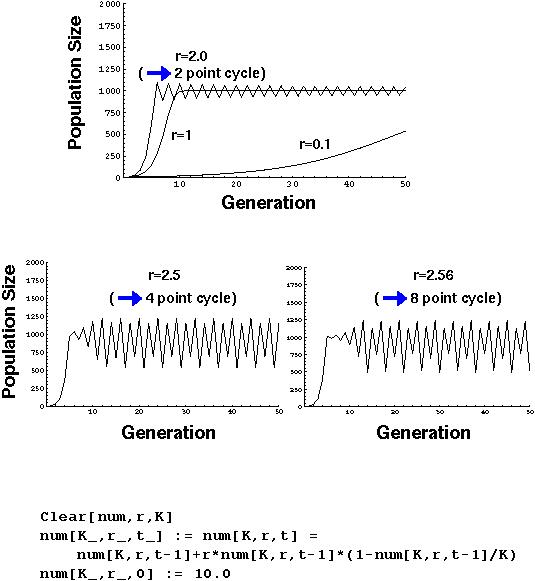
Logistic Growth Model (Discrete)
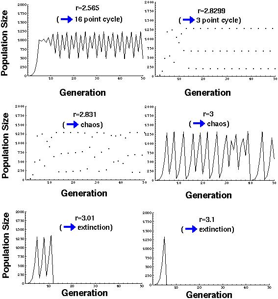
The dynamics of the logistic equation are bizarre to say the least.
The periodic cycles and the chaotic fluctuations may not, however, be particularly relevant.
Hassell (1976) studied 28 insect populations. 26 of them exhibited values of r leading to a stable equilibrium point, one led to a periodic cycle (the Colorado potato beetle), and only one led to chaotic behavior (blowflies under laboratory conditions).
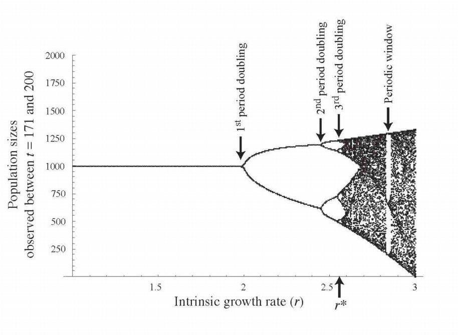
Logistic Growth Model (Discrete)
Bifurcation Diagram
Logistic Growth Model (Continuous)
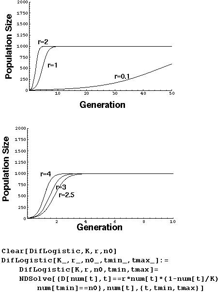
The logistic model is extremely sensitive to the manner in which it is modeled. The continuous and discrete time formulations agree when r is small, but lead to completely different predictions when r is large!
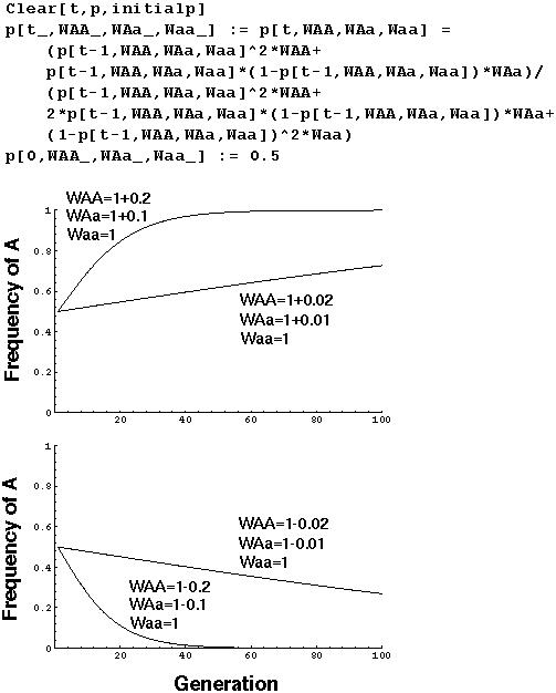
Haploid Selection Model (Discrete)
In this model, there are only two parameters to chose: WA and Wa.
There are therefore two main cases: WA > Wa or WA < Wa.
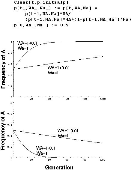
Haploid Selection Model (Continuous)
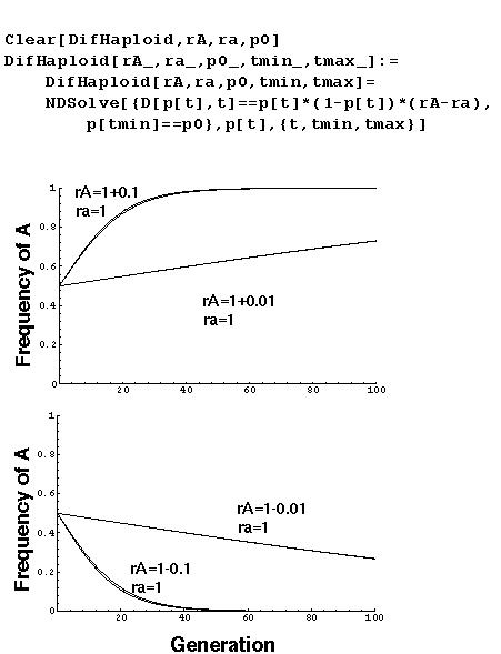
The continuous and discrete time models correspond extremely well.
When rA > ra (or WA > Wa), the frequency of A increases over time.
When rA < ra (or WA < Wa), the frequency of A decreases over time.
Diploid Selection Model (Discrete)
In this model, there are three parameters to chose: WAA, WAa, and Waa.
These are broken into four categories:
- WAA > WAa > Waa (Directional selection favoring A)
- WAA < WAa < Waa (Directional selection favoring a)
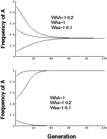
- WAA < WAa > Waa (Heterozygote advantage or overdominance)
- WAA > WAa < Waa (Heterozygote disadvantage or underdominance)
Diploid Selection Model (Discrete)
The behavior of the four fitness categories appears to be:
- WAA > WAa > Waa (Fixation on A)
- WAA < WAa < Waa (Fixation on a)
- WAA < WAa > Waa (Polymorphic equilibrium)
- WAA > WAa < Waa (Fixation on A or a)
Remember: These are inferences from just a few graphs using just a few starting conditions and fitness values.
 Back to biology 301 home page.