
One-Locus Selection Models
After one generation of random mating in a single large population with no selection and no mutation, genotype frequencies at a diploid autosomal locus become:
 Hardy-Weinberg equilibrium.
This is true regardless of whether there is random mating among gametes or random mating among individuals.
Furthermore,
Allele frequencies do not change over time.Question: What if there are fitness differences between the genotypes?
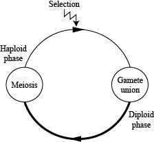
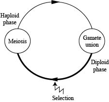
We will start (CENSUS) at the beginning of the haploid phase.
Let there be two haploid genotypes (A and a) with
What is the frequency of A at this point? p[t] =
After selection has occurred (before reproduction), how many A individuals will still be alive on average?
How many a individuals will still be alive on average?
What is the frequency of A among these adults?
This will also be the frequency of the A allele among the gametes produced by the haploid adults.
These gametes unite at random and undergo meiosis (neither of which will change the allele frequencies) to produce the next generation of haploids.
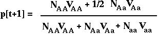
Therefore, in the next generation, the frequency of the A allele is:
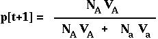
 RECURSION giving the allele frequency over time in the haploid model with viability selection.
(The denominator in this equation is the mean ABSOLUTE fitness of the population.)
For instance, it may be known that a individuals are twice as likely to die.
After selection, we don't know the exact number of individuals in the population of each type, but we know that they are in the following ratios:
which is equivalent to
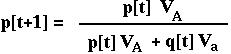
Given these ratios, the frequency of the A allele is
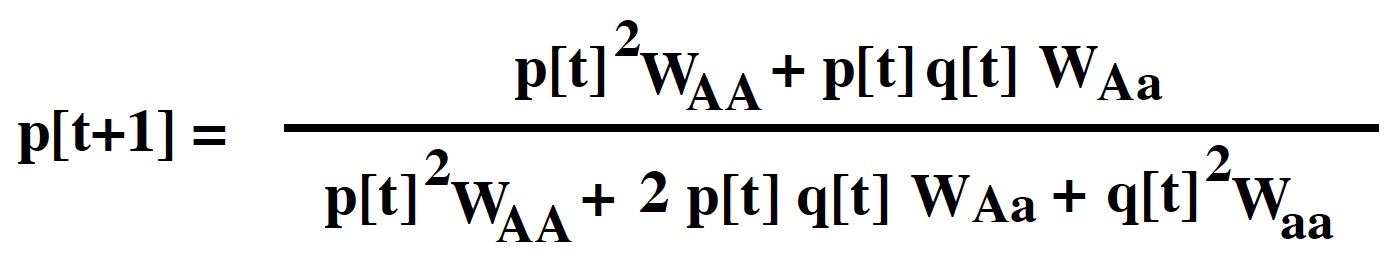
This has the same form as the equation with absolute viabilities, but can be used more generally.
(The denominator in this equation is the mean RELATIVE fitness of the population.)
Note: Since q[t]=1-p[t], this is a function in terms of one variable, p[t], and two viability parameters.
We continue to assume no migration, no mutation, a large randomly mating population, and discrete generations.
With either random union of gametes in a gamete pool or with random mating of individuals, the diploid offspring are in Hardy-Weinberg proportions: p2[t] : 2 p[t] q[t] : q2[t], where p[t] is the frequency of the A allele among the mating individuals in generation t.
We will start (CENSUS) at the beginning of the diploid stage.
What is the frequency of A at this point? p[t] =
Not all diploid individuals survive to reproduce:
After selection has occurred (before reproduction), how many AA individuals will still be alive on average?
How many Aa individuals will still be alive on average?
How many aa individuals will still be alive on average?
What is the frequency of the A among these adults?
These gametes unite at random (which will not change the allele frequencies) to produce the next generation of diploids.
Therefore, in the next generation, the frequency of the A allele is:
Substituting p2[t] N for NAA, etc, we can rewrite this as:
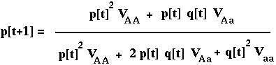 RECURSION giving the allele frequency over time in the diploid model with viability selection.
Again, any relative measure of viability can be used rather than absolute measures:
The adults after selection will then be in the following proportions:
This tells us that the ratio of A to a alleles will be
The frequency of the A allele among adults is therefore:
For populations with overlapping generations, a similar model may be constructed in continuous time.
We now define fitness according to the growth rate of each genotype:
These definitions tell us that
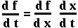
Mathematical Aside: The chain rule
A function of one variable, f(x), obeys the one-variable chain rule:
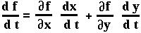
Now since p is a function of both NA and Na, we can use the two-variable chain rule to determine what dp/dt equals (on board).
dp/dt = p (1-p) (rA-ra)
(rA-ra) is the selective advantage of allele A in terms of its growth rate.
A similar equation can be derived for the diploid model of selection in continuous time, but we will not study this equation in class.
Not really. Discrete and continuous time models generally behave in a similar fashion when changes occur slowly over time.
For this model of selection, this implies that they will be similar when the fitnesses are near one in the discrete model.
This is fairly easy to prove (on board), although we will need the following facts:
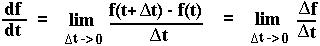
Mathematical Aside: Definition of the derivative
Mathematical Aside: Approximating the fraction 1/(1+x)
If x is very small, then 1/(1+x) is approximately 1-x.
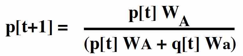
When selection is weak, the allele frequency changes over time in the discrete model may be described approximately by the differential equation:
dp/dt = p (1-p) s
where s = WA-Wa. This is the same equation governing the change in allele frequency over time in the continuous time model, if we define s = rA-ra.
 Back to biology 301 home page.