
Continuous Probability Distributions
One interesting point about continuous probability distributions is that, because an infinite number of points lie on the real line, the probability of observing any particular point is effectively zero.
Continuous distributions are described by probability density functions, f(x), which give the probability that an observation falls near a point x:
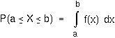
One can therefore find the probability that a random variable X will fall between two values by integrating f(x) over the interval:
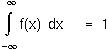
The total integral over the real line must equal one:
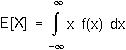
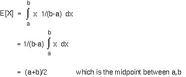
As in the discrete case, E[X] may be found by integrating the product of x and the probability density function over all possible values of x:
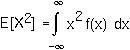
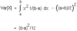
The Var(X) equals E[X2] - (E[X])2, where the expectation of X2 is given by:
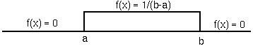
The expected value of the uniform distribution equals:
It's variance equals:
Example: Say that a particular chromosome is mapped out to be 2 morgans long. This chromosome is observed in several meiotic cells. Among those chromosomes containing a single cross-over, the mean position of the cross-over is 1 morgan from an end, but the variance is 1/2. Is this variance higher or lower than expected? What might cause such an observation?
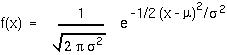
Where  is the mean and
  2 is the variance of the distribution. (The mean, for example, may be found by integrating x f(x) over all values of x.)
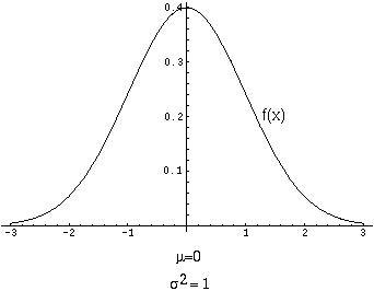
Gauss and Laplace noticed that measurement errors tend to follow a normal distribution.
Quetelet and Galton observed that the normal distribution fits data on the heights and weights of human and animal populations. This holds true for many other characters as well.
Why does the normal distribution play such a ubiquitous role?
The Central Limit Theorem For independent and identically distributed random variables, their sum (or their average) tends towards a normal distribution as the number of events summed (or averaged) goes to infinity.
For example, as n increases in the binomial distribution, the sum of outcomes approaches a normal distribution:
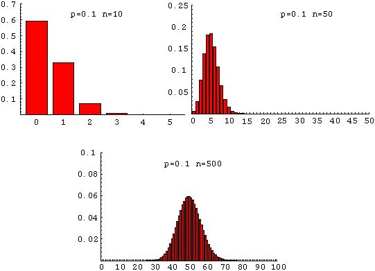
In particular, we expect that if several genes contribute to a trait, the trait should have a normal distribution. [The random variable that is being summed or averaged is the contribution of each gene to the trait.]
 , then the time until the first event occurs has an exponential distribution:
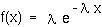
This is the equivalent of the geometric distribution for events that occur continuously over time.
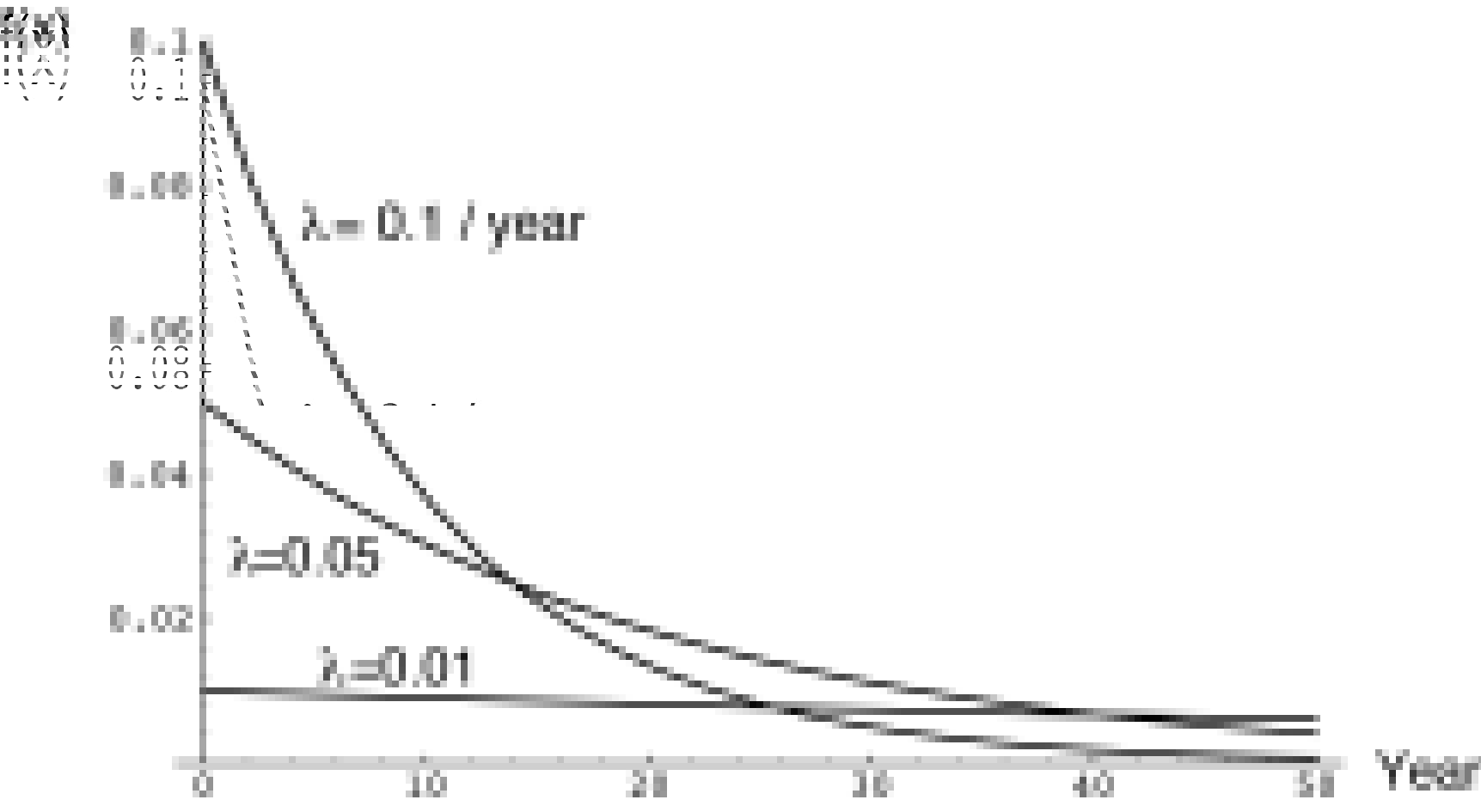
E[X] can be found be integrating x f(x) from 0 to infinity, leading to the result that E[X] = 1/.
The variance of the exponential distribution is 1/2.
For example, let equal the instantaneous death rate of an individual. The lifespan of the individual would be described by an exponential distribution (assuming that does not change over time).
:
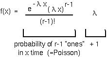
The mean of the gamma distribution is r/ and the variance is r/2.
Example: If, in a PCR reaction, DNA polymerase synthesises new DNA strands at a rate of 1 per millisecond, how long until 1000 new DNA strands are produced? (Assume that DNA synthesis does not deplete the pool of primers or nucleotides in the chamber, so that each event is independent of other events in the PCR chamber.)
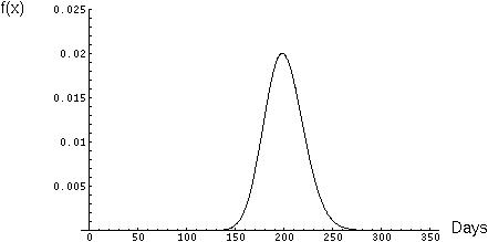
You could answer them by integrating the gamma distribution from 0 up until 95% of the area under the curve is covered. The answer in this case would be 234 days.
Or you could answer them by saying that because of the Central Limit Theorem, the distribution of the number of days should be approximately normal with mean r/ and variance r/2.
By using a statistical table, you figure out that the upper 95% confidence limit is 1.65 standard deviations above the mean. In this case, your estimate would be 200 + 1.65*Sqrt(400) = 233 days. (Pretty good!)
Either way, you tell your committee not too worry, it shouldn't take you much longer than 200 days to collect your data.
 Back to biology 301 home page.