Spread of Disease

In this lecture, we'll work through a non-linear model based on a paper by Anderson and May (1982).

The problem is briefly described in Edelstein-Keshet, p. 65:

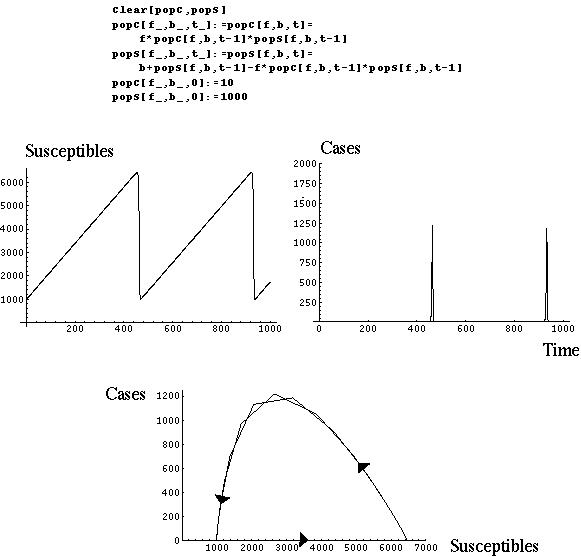
[Anderson and May] suggest a simple discrete model for the spread of disease that demonstrates how regular cycles of infection may arise in a population.
Taking the average period of infection as the unit of time, they write equations for the number of disease cases C_t and the number of susceptible individuals S_t in the tth time interval.
They make the following assumptions:
(i) the number of new cases at time t+1 is some fraction f of the product of current cases C_t and current susceptibles S_t;
(ii) a case lasts only for a single time period;
(iii) the current number of susceptibles is increased at each time unit by a fixed number B (B does not equal 0) and decreased by the number of new cases;
(iv) individuals who have recovered from the disease are immune.

Based on this description of the model, we will determine the equations for C_t+1 and S_t+1, determine the equilibria of these equations, and analyse the stability of the equilibria.

Spread of Disease

Convince yourself that the recursions may be written as:

C_t+1 = f C_t S_t

S_t+1 = S_t + B - f C_t S_t

The equilibria of these equations must solve both of the following equations:

C = f C S

S = S + B - f C S

The first equation tells us that either C=0 or S=1/f at equilibrium.

The second equation tells us that if C=0 then S will not remain constant (the number of susceptibles would increase by B every time unit), while if S=1/f then both equations will be satisfied if C=B.

We conclude that there is only one equilibrium (or steady state) of this model with the number of susceptible individuals equal to S=1/f and the number of current cases equal to C=B.

Remember that there is also another class of immune individuals in the population, but these are considered to be outside the system.

Spread of Disease

We now do a local linear stability analysis around this equilibrium.

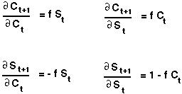
First we find the partial derivatives of the two equations:

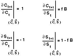
Then we evaluate these partial derivatives at the equilibrium:

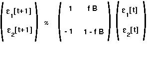
Finally we plug these values into the local stability matrix which approximates the dynamics near the equilibrium:

Spread of Disease

To find the eigenvalues, take the determinant of this matrix minus

times the identity matrix.

This gives the characteristic polynomial:

(1-

) (1 - f B -

) + f B = 0

² -

(2 - f B) + 1 = 0

The two eigenvalues must solve this polynomial.

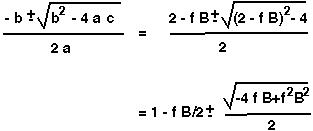
We use the quadratic formula to find that

There are two cases which we must consider.

(1) The term in the squareroot is positive if f B > 4. In this case,

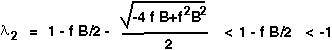
so the second eigenvalue will be less than -1. We therefore predict oscillations around the equilibrium that grow in magnitude over time.

Spread of Disease

(2) The term in the squareroot is negative if f B < 4. In this case, we have complex eigenvalues.

Mathematical Aside: Complex eigenvalues in a discrete model.

Consider a dynamical system whose leading eigenvalues are given by the complex conjugate pair:

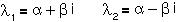
These eigenvalues indicate that the system will undergo a counter-clockwise rotation every generation by an amount and will be "stretched" by a factor ||, where:

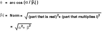
Whether these cycles will spiral into or away from the equilibrium depends, in a discrete model, on the stretching factor or norm.

If the stretching factor (||) is greater than one, then the system will spiral away from the equilibrium (UNSTABLE EQUILIBRIUM) and if it is less than one, it will spiral inwards (STABLE EQUILIBRIUM).

In this case,

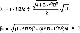
Therefore, since the norm of the complex eigenvalues is exactly equal to one, we expect the system to cycle around the equilibrium without any strong tendency to cycle inwards or outwards.

Spread of Disease

Values for the parameters given by Anderson and May are B = 12 births/1000 individuals (UK) and f=0.0003.

Using these numbers, f B < 4, and we expect to see cycling:

Back to biology 301 home page.