Review: Stability analysis in one-variable models

The next step is to determine when the various equilibria are STABLE and when they are UNSTABLE (at least locally).

We have already learned how to perform a local stability analysis for a single non-linear equation in one variable. Let's review.

DISCRETE MODEL

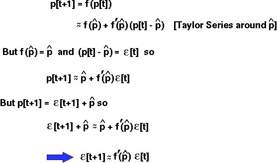
Say that the population is currently a small distance () away from the equilibrium. We use the Taylor Series to determine whether this perturbation will grow or shrink.

Let f(p[t]) be the recursion equation giving p[t+1] as a function of p[t]. Then:

Review: Stability analysis in one-variable models

• grow over time if |f'()| > 1

• shrink over time if |f'()| < 1

• stay on the same side of the equilibrium (non-oscillatory) if f'() > 0

• flip from side to side of the equilibrium (oscillatory) if f'() < 0

|f'()| < 1

We also learned how to do a local stability analysis for a one-variable model in continuous time. In that case, we found that a perturbation would

• have a positive rate of change and grow if f'() > 0

• have a negative rate of change and shrink if f'() < 0

f'() < 0

How do we generalize this to a system of equations in more than one variable???

In the following, we will focus on a system of equations in discrete time. To learn how to analyse the stability of an equilibrium for a system of equations in continuous time, read Roughgarden pp. 572-577.

Stability analysis in multiple-variable models

First of all, we have to learn how to do the Taylor Series when we have more than one variable.

Mathematical Aside: Taylor Series in Multiple Variables

Let x₁[t+1] be written as some function (f₁) of all the variables in the previous generation: f₁(x₁[t],x₂[t],...x_n[t]). The Taylor Series of this equation is:

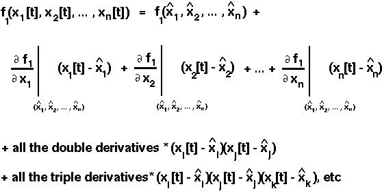
Notice that if we only had one variable (x₁[t]), then the Taylor Series would be the same as before.

Stability analysis in multiple-variable models

To make the Taylor Series more useful for our purposes, let's assume that the population is near an equilibrium point. This will allow us to ignore the double derivatives and higher derivatives, since these are multiplied by very very small terms (squares and higher of terms).

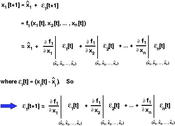
Then:

PHEW!

This last equation gives us the perturbation of the first variable from its equilibrium value in the next generation as a function of the partial derivatives of f₁ and the perturbations of all the variables in the previous generation.

The perturbation of the second variable will be described by a similar equation, except that f₁ would be replaced by f₂, etc.

NOTICE: What we have done is taken the NON-LINEAR equations (f₁, f₂, ... , f_n) and turned them into LINEAR APPROXIMATIONS near the equilibrium we are interested in.

Stability analysis in the Lotka-Volterra model

In the Lotka-Volterra competition model with two species, we have two recursion equations which are:

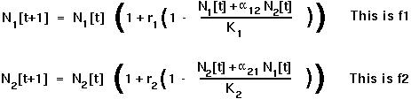
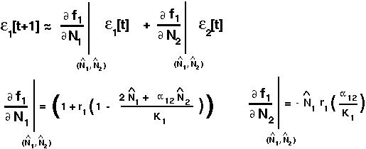
The Taylor Series of the first one gives:

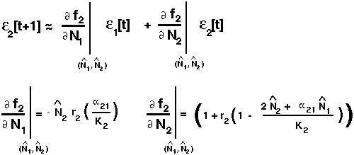
and the Taylor Series of the second one gives:

Stability analysis in the Lotka-Volterra model

Now we're ready for business.

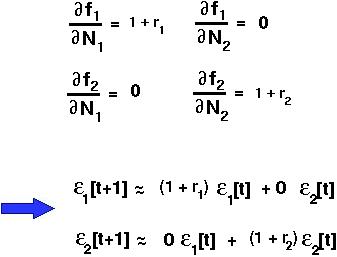
There are four possible equilibria whose stability we want to determine. First, let's work on the simplest one with both N₁ and N₂ equal to zero (both populations are extinct).

Both species extinct at equilibrium

This can be written in MATRIX form:

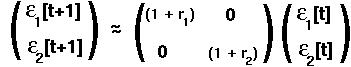
From what we know about matrices, when will this perturbation vector grow over time?

If the leading eigenvalue is greater than one!

But the eigenvalues in this case are (1+r₁) and (1+r₂).

• If either r₁ or r₂ is greater than zero, the leading eigenvalue will be greater than one and the equilibrium with neither species present is locally UNSTABLE.

• If both r₁ and r₂ are smaller than zero, the leading eigenvalue will be less than one and the equilibrium with neither species present is locally STABLE. [Note that (1+r₁) and (1+r₂) will not be negative since an individual cannot have negative offspring.]

Stability analysis in the Lotka-Volterra model

Species 2 extinct at equilibrium and species 1 at K₁.

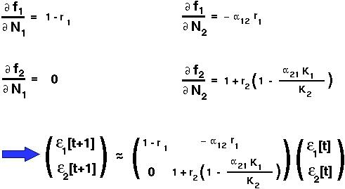
The two eigenvalues of this matrix are (1-r₁) and (1 + r₂ (1- K₁/K₂)).

Both of these eigenvalues must be less than one for the equilibrium to be stable.

• r₁ must lie between 0 and 2 for the equilibrium with N₁ = K₁ to be stable (as in logistic).

• If r₂ is positive and K₂ is greater than K₁, then the second eigenvalue will be greater than one and the equilibrium will be unstable. [Note that the second eigenvalue will not be negative since it equals the number of offspring of an individual of species 2 when species 2 is rare and species 1 is at its carrying capacity.]

Stability analysis in the Lotka-Volterra model

Species 1 extinct at equilibrium and species 2 at K₂.

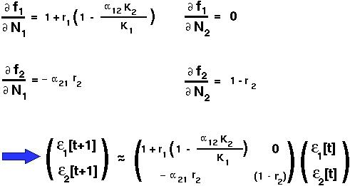
The two eigenvalues of this matrix are (1-r₂) and (1 + r₁ (1- K₂/K₁)).

Both of these eigenvalues must be less than one for the equilibrium to be stable.

• r₂ must lie between 0 and 2 for the equilibrium with N₂ = K₂ to be stable (as in logistic).

• If r₁ is positive and K₁ is greater than K₂, then the second eigenvalue will be greater than one and the equilibrium will be unstable. [Note that the second eigenvalue will not be negative since it equals the number of offspring of an individual of species 1 when species 1 is rare and species 2 is at carrying capacity.]

Stability analysis in the Lotka-Volterra model

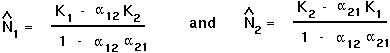
Both species present at equilibrium.

The equilibria in this case are:

The partial derivatives evaluated at this equilibria are now:

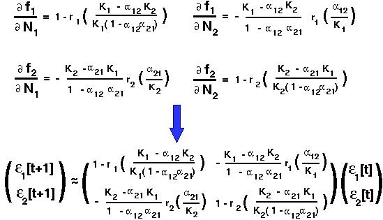
The two eigenvalues of this matrix are extremely complicated.

Stability analysis in the Lotka-Volterra model

In this case, the eigenvalues are (1-r) and .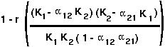

For the first eigenvalue to be less than one in magnitude, r must lie between 0 and 2 (similar to logistic).

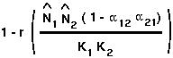
The second eigenvalue is easier to interpret when written in terms of and :

.

If competition is so strong that (1 - ) is negative, the second eigenvalue will be greater than one in magnitude even if the two species have positive intrinsic growth rates (r).

Strong competition prevents two species from stably co-existing.

With weak competition, (1 - ) > 0, the equilibrium numbers of species 1 and species 2 will be positive only if K₁ > K₂ and K₂ > K₁.

Under these conditions,

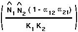
is positive and less than one in magnitude. Hence, if the first eigenvalue is less than one in magnitude (i.e. 0 < r < 2), then the second eigenvalue will also be.

Weak competition allows two species to co-exist, but only if their growth rates are positive and less than two.

We will talk about how these conditions were obtained and also how to analyse the model when r₁ does not equal r₂ in class.

In summary:

The equilibrium without either species is stable if r₁ and r₂ are both negative.

The equilibrium with only species 1 present is stable if 0 < r₁ < 2 and K₂ < K₁.

The equilibrium with only species 2 present is stable if 0 < r₂ < 2 and K₁ < K₂.

Assuming r₁ = r₂, the equilibrium with both species present is stable if 0 < r < 2 and (1 - ) > 0, which implies that K₁ > K₂ and K₂ > K₁ for the equilibrium numbers to be positive.

Back to biology 301 home page.