
Introduction to Demography
To study changes in populations with age or stage structure requires demographic theory, which relates probabilities of survival and reproduction at each age to the growth and composition of a population.
Today we'll introduce some of the concepts and parameters important in studying the age structure and growth of a population.
We'll focus on the demography of Canada. I obtained the data primarily from census data published by Statistics Canada (catalogs 84-210, 84-211, 91-213-XPB) and from the International Database maintained by the US Census Bureau.
(Other web sites of interest are:
Total Population Size:
Consider a population measured at particular points in time, for instance every five years during a census. One can track the population size from census to census to get a historical perspective on population growth:
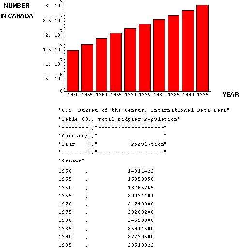
This shows that Canada has grown in the recent past. For instance, between the 1990 and 1995 censuses, the population grew by 1.3% per year (although about half of this growth was due to migration).
In studying a natural population, there are many complications that we are going to ignore. For instance, we are going to ignore problems associated with emigration (out of the population) and immigration (into the population). Furthermore, males and females generally differ in their demographic parameters but we're going to focus on females.
We'll use five year census points and base our analysis on the 1991 census, so that we may compare our projections to the 1996 census data.
Age Distribution:
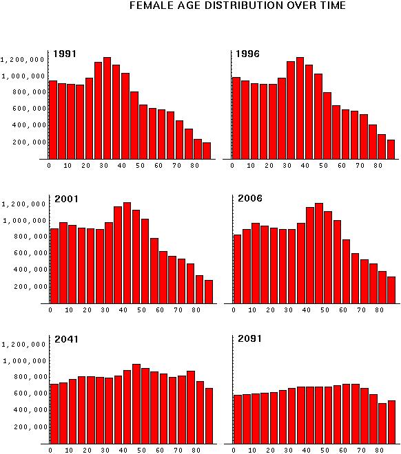
A population can be described by how many individuals there currently are in each age class.
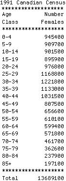
By convention, the number of females at time t in age class x is nx,t.
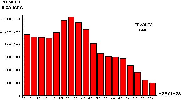
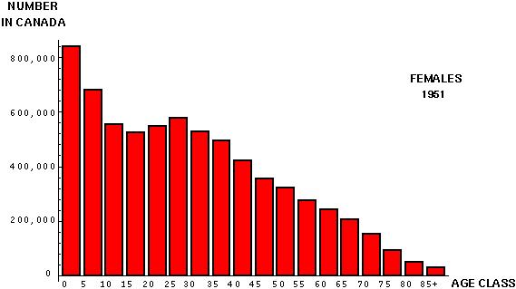
Interestingly, this age distribution has changed substantially since 1951:
Mortality:
Another critical piece of data that we can get from the census is how many individuals die per year, by age class:
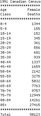
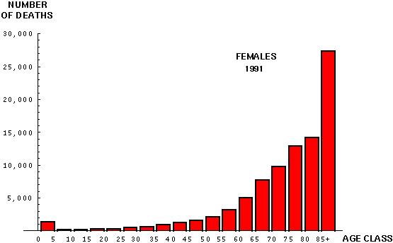
Generally, the number of deaths in the population is less useful than the proportion of individuals in each age class that die between each census period.
The proportion of individuals in each age class that die between each census period is obtained by multiplying the number that died per year by the length of the age class and dividing by the total number of individuals in each age class:
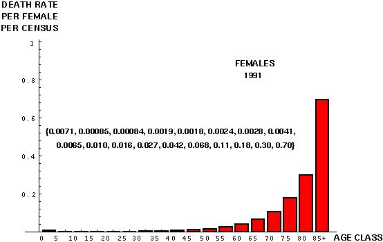
The probability of dying from age class x to age class x+1 is denoted by dx.
Another important parameter is the probability of surviving from age class x to age class x+1, px, which is simply 1-dx.
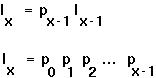
Sometimes, survival data are given from birth to the current age class. The probability of surviving from birth to the beginning of age class x is generally written as lx.
Fortunately, one can determine lx from px and vice versa, using the fact that:
Fertility:
Finally, we must determine the number of babies that individuals in each age class have:
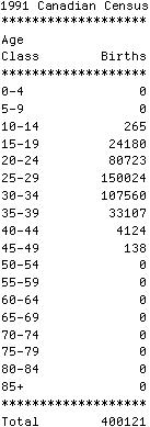
These figures are for all births. We are following females, however, and only 195,916 of these births (48.96%) were girls. [A male-biased sex ratio at birth is a general phenomenon among humans.] We'll use this proportion to esimate the number of female offspring born in 1991 to mothers in each age class.
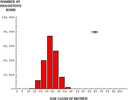
Again, the total number of daughters born is less useful than the number of daughters born per female in each age class during the census period.
This is obtained by multiplying the number of daughters born by the length of the age class and dividing by the total number of females in each age class:
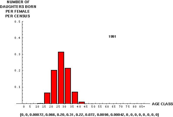
The number of female offspring per female in age class x is denoted by mx.
Notice that the total period fertility rate ( mx) is only 0.88. That is, even if all females survive from birth until the end of their reproductive period, the number of females born to a cohort of women will not fully replace that cohort.
With these parameters of a population in hand, we can turn next to analysing how a population will change over time.
In summary, we have a whole bunch of data about the Canadian population, from which we can infer:
Following Hastings, we will assume that individuals censused within an age class are actually at the beginning of that age class.
In particular, the number of individuals within the 0-4 age class will be the total number of individuals born since the previous census. The number of individuals in the 5-9 age class will then be those that were in the 0-4 age class and that survived as 0-, 1-, 2-, 3-, and 4-year olds.
Other texts make different assumptions, e.g. that censused individuals are at the end of their age class.
Step 1: The first step is to determine the transition matrix for the population from census point to census point.
First, the females in age class x reproduce (at rate mx). The females then move up to age class x+1 if they survive to the next census (with probability px ).
Therefore, given the population composition at census t, at census t+1
nx,t mx
(2) the number of individuals in other age classes is nx-1,t px-1
(3) the number of individuals in the last age class ( ) is n-1,t p-1 + n,t p, since some individuals live past 90.
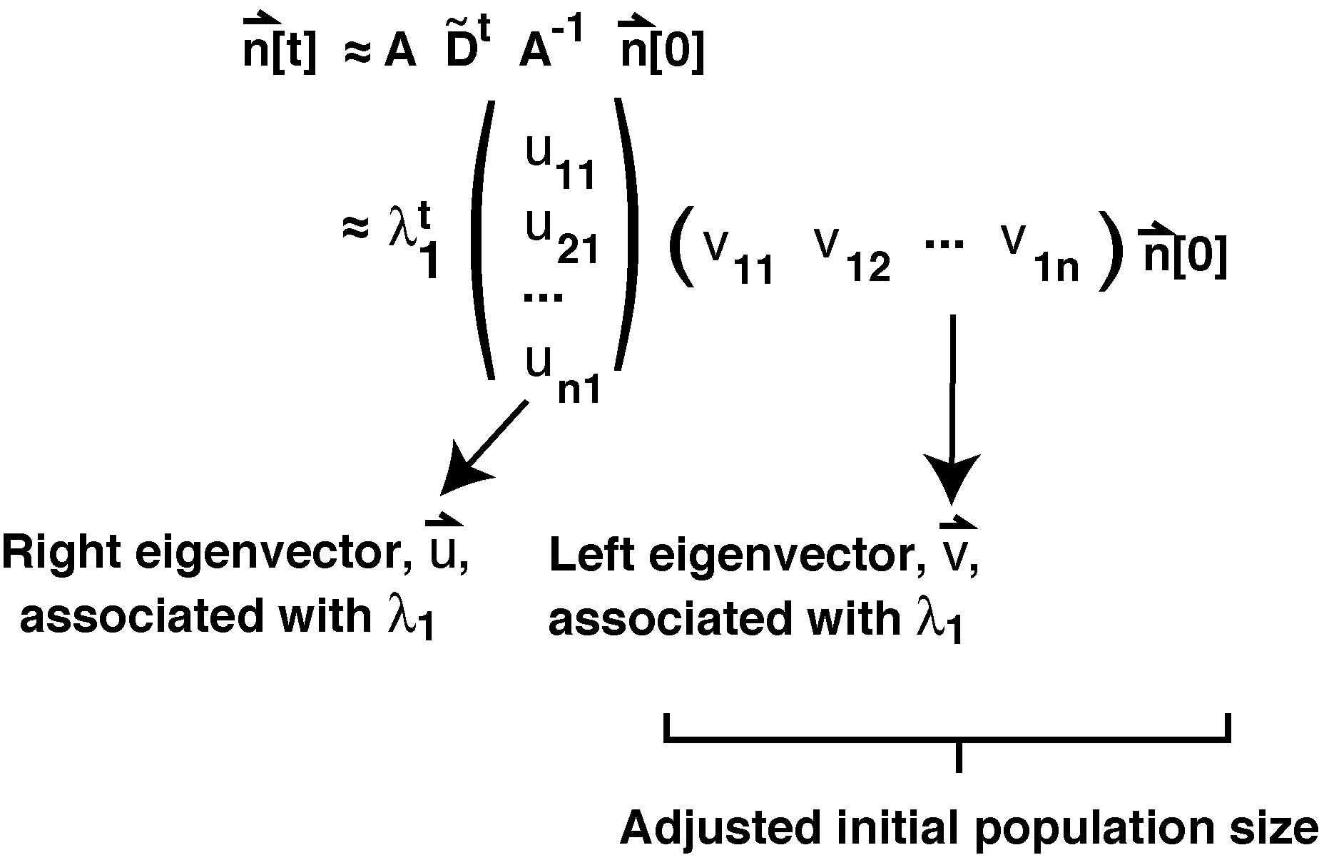
Population changes can more easily be described using matrix notation:
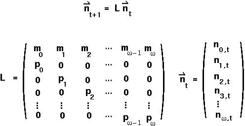
L is known as a Leslie Matrix for population projection.
We can then proceed through our steps to find the general solution:
Step 2: Determine the eigenvalues of the Leslie matrix.
Step 3: Make a diagonal matrix, D, with one eigenvalue in each of the diagonal positions.
Step 4: Determine the eigenvectors associated with each eigenvalue.
Step 5: Make a transformation matrix, A, whose columns are the eigenvectors (placed in the same order as the eigenvalues in matrix D).
Step 6: Write the general solution of the linear equations as:
For large matrices, however, this can be a real mess! So we will use a simpler approximation.
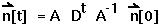
If we place the leading eigenvalue (i.e. the eigenvalue with largest magnitude) in the first position, Dt will become more and more similar over time to the following matrix:
That is, because  1 is larger than all the other eigenvalues, 1t will be much larger than it (for i other than 1), and the influence of these other eigenvalues will become negligible after enough time has passed.
Note: Whether or not this will give a sufficiently accurate approximation depends on how much time has passed and on whether the other eigenvalues are near the leading eigenvalue in magnitude.
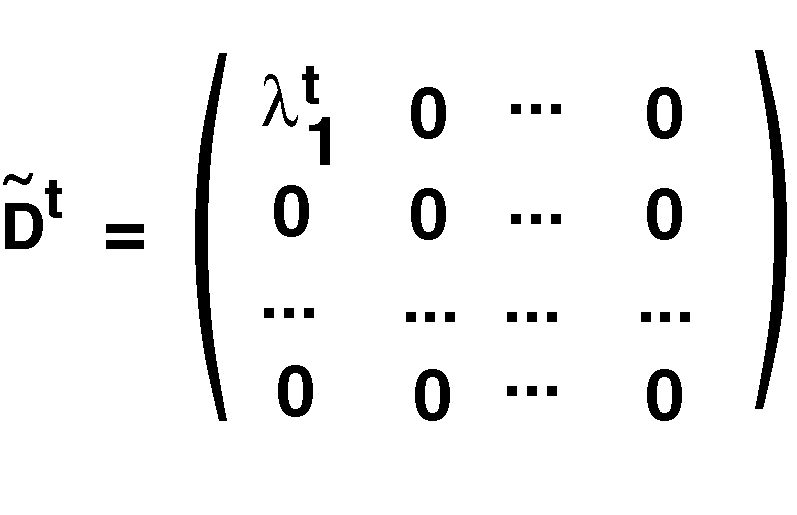
An approximate projection of the population is then:
where ![]() is the first column of the A matrix and
is the first column of the A matrix and ![]() is the first row of the A-1 matrix.
is the first row of the A-1 matrix.
Note: The first column of A is also called the right eigenvector, which must solve L![]() =
= ![]() . Similarly, the first row of A-1 is called the left eigenvector, which must solve
. Similarly, the first row of A-1 is called the left eigenvector, which must solve ![]() L =
L = ![]() . To use this approximate solution, the length of the left eigenvector must be adjusted so that
. To use this approximate solution, the length of the left eigenvector must be adjusted so that ![]()
![]() = 1.
= 1.
The left eigenvector contains information about the "reproductive value" of each age class. When multiplied by the initial population vector, it gives the initial population size adjusted for the fact that some age classes (e.g., teenagers) have greater reproductive value than others (e.g., post-menopausal).
Once the general solution is found, the iteration is simple: just multiply by 1 every generation.
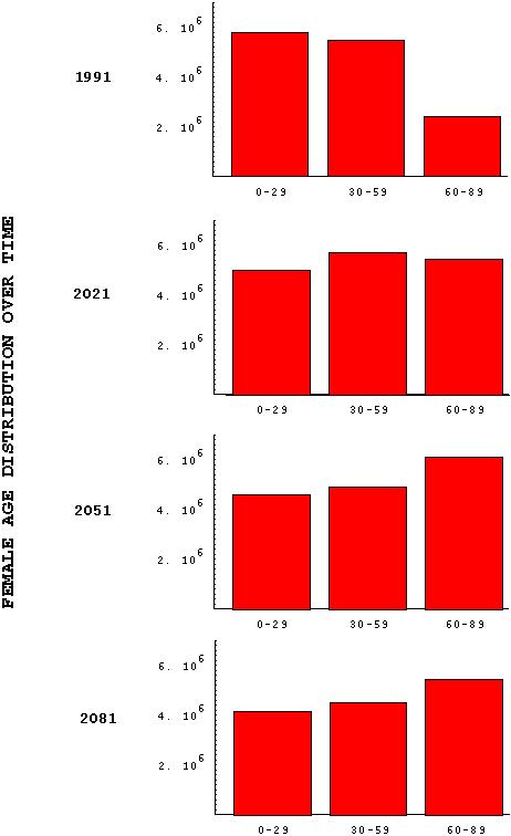
Let's first analyse the Canadian data using a simplified version of the census data.
We'll group ages from 0-29, 30-59, and 60+ to get only three classes. Note that the analysis will be less accurate with fewer age classes.
The general Leslie matrix for this case would be:
For the Canadian population, I get:
p = {0.9851, 0.9348, 0.1399}
n1991 = {5798100, 5460500, 2430500}
 to get:
n2051 = {4618060, 4931180, 6101160} [in two censuses]
n2081 = {4159900, 4549370, 5463250} [in three censuses]
This indicates that the proportion of females in the oldest age class (60+) should have risen rapidly from 18% in 1991 to 34% in 2021 to 39% in 2051, where it should remain roughly constant.
It also indicates that the population size of females should have grown by 18% between 1991 and 2021, but decrease by 3% between 2021 and 2051, decrease by 9% between 2051 and 2081, and by roughly 9% every 30 years thereafter.
Currently, the population is very young and is growing more rapidly because of this. As the Canadian population ages, its growth rate will decline.
Let's now use the simpler method described above, where we assume that the leading eigenvalue dominates the system.
For this matrix, the eigenvalues are {0.9064, -0.3231, 0.1399}.
After an initial period of time, a linear system will approach a stable distribution, where the ratio of individuals in each class is constant and given by the right eigenvector associated with the leading eigenvalue.
In this case, the right eigenvector associated with the leading eigenvalue is: ![]() =
{0.2931, 0.3185, 0.3884} [This eigenvector has been normalized to sum to one.]
=
{0.2931, 0.3185, 0.3884} [This eigenvector has been normalized to sum to one.]
In demography, this distribution is known as the STABLE AGE DISTRIBUTION.
Once at the stable age distribution, every age class and hence the whole population will be multiplied by the leading eigenvalue every census.
In this example, the leading eigenvalue is 0.9064, indicating that the population will shrink by 9.36% every census.
We can then use these values to project the population into the future.
Adjusting the initial population vector by the reproductive value gives ![]() n1991 = 1.91 107. This is larger than the female population size in 1991 of 1.37 107, because the 1991 population is fairly young relative to the stable age distribution.
n1991 = 1.91 107. This is larger than the female population size in 1991 of 1.37 107, because the 1991 population is fairly young relative to the stable age distribution.
Our estimates of the future population are then  t times the stable age distribution,
 ![]() =
{0.2931, 0.3185, 0.3884}, times the adjusted initial population size of 1.91 107.
=
{0.2931, 0.3185, 0.3884}, times the adjusted initial population size of 1.91 107.
n2051 = {4596840, 4995890, 6092580} [in two censuses]
n2081 = {4166750, 4528460, 5522540} [in three censuses]
This correctly predicts that the proportion in the oldest age class (60+) should be 39%.
This approximation suggests that the population size of females should grow by 26% (rather than 18%) between 1991 and 2021, then decrease by 9% (rather than 3%) between 2021 and 2051, and then decrease by 9% every 30 years thereafter.
Although this method should technically only work well for longer time periods, it still does very well in this case even over the short time period measured here.
After only two censuses, the approximate method performs nearly as well as the recursions using the full Leslie matrix. There is a short, initial phase, however, in which the non-leading eigenvalues still exert an influence on the population dynamics.
The phase is particularly short in this example, since the non-leading eigenvalues are all small (-0.3231 and 0.1399) and so these terms rapidly become negligible in the general solution.
In summary: the leading eigenvalue does estimate long term growth, its right eigenvector does estimate the long term ratio between classes, but the short term growth can be influenced by the fact that the population isn't yet at a stable age distribution.
The above analysis with only three age classes provides only a crude demographic picture of the Canadian population.
Let's now return to an analysis using the full data matrix.
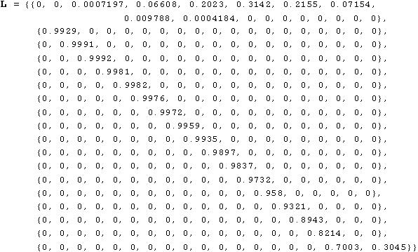
This is an example where Mathematica comes in really handy!
The leading eigenvalue for this matrix is 0.9772.
It's right eigenvector gives the stable age distribution: ![]() =
{0.05059, 0.05140, 0.05256, 0.05374, 0.05489, 0.05607,
0.05724, 0.05841, 0.05953, 0.06052, 0.06130, 0.06171,
0.06146, 0.06025, 0.05747, 0.05260, 0.04422, 0.04603} (normalized to sum to one).
=
{0.05059, 0.05140, 0.05256, 0.05374, 0.05489, 0.05607,
0.05724, 0.05841, 0.05953, 0.06052, 0.06130, 0.06171,
0.06146, 0.06025, 0.05747, 0.05260, 0.04422, 0.04603} (normalized to sum to one).
This tells us many things. There will about 5.1% of the population under age 5 at the stable age distribution and 20.8% under age 20. Similarly, there will be 20.0% of the population over age 70 and 32.2% over age 60.
We can compare these figures to their 1991 values of 9.2% of the population over age 70 and 17.8% over age 60, to infer that the population will in the future be composed of nearly twice as many older individuals then there were in 1991, expressed as a fraction of the population.
Furthermore, when the population does reach the stable age distribution, it will shrink by 2.28% during every five year census period.
The left eigenvector of reproductive values is
![]() =
{3.2481, 3.1968, 3.1265, 3.0554, 2.7764, 2.0597, 0.9944, 0.2724,
0.0339, 0.0014, 0, 0, 0, 0, 0, 0, 0, 0} (normalized so that
=
{3.2481, 3.1968, 3.1265, 3.0554, 2.7764, 2.0597, 0.9944, 0.2724,
0.0339, 0.0014, 0, 0, 0, 0, 0, 0, 0, 0} (normalized so that ![]()
![]() = 1). When multiplied by the vector of female population size from 1991, the adjusted initial population size becomes
= 1). When multiplied by the vector of female population size from 1991, the adjusted initial population size becomes ![]() n1991 = 1.82 107 (again larger than the initial female population size of 1.36 107).
n1991 = 1.82 107 (again larger than the initial female population size of 1.36 107).
Taking this adjusted initial population size, 1.82 107, and multiplying by the stable age distribution times (0.9772)t provides an estimate of the female age distribution in future censuses.
Of course, with Mathematica, it is straightforward to iterate the Leslie matrix to predict future population states.
Finally, we can do a check by comparing the expected age distribution in 1996 to the actual census:
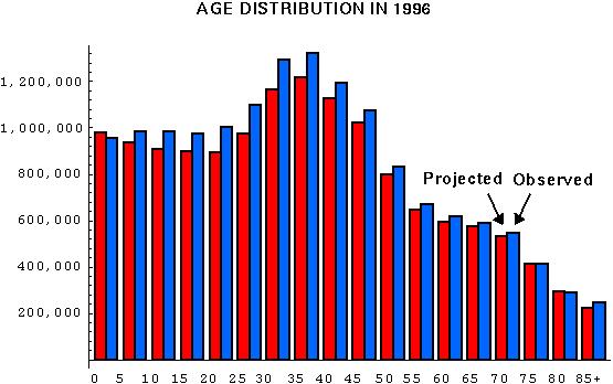
This comparison shows that our projection falls short a bit. Firstly, the actual population growth was 10.4% over this five year period whereas the Leslie matrix projection estimated only 3.9% growth. Secondly, the shapes of the two age distributions are different.
These discrepancies are due to three main factors: (1) immigration and emigration, (2) too coarse an age distribution, and (3) a changing life table. In fact, we know that the net immigration rate over this time period was approximately 500,000 females. Furthermore, the birth rate has continued to drop over this period, especially for women under 30.
 Back to biology 301 home page.