Biology 301

Solving Linear Equations: Red Blood Cell Production

Aim: To use matrix notation to determine how the number of red blood cells varies over time (from Edelstein-Keshet 1988).

"In the circulatory system, the red blood cells (RBCs) are constantly being destroyed and replaced. Since these cells carry oxygen throughout the body, their numbers must be maintained at some fixed level. Assume that the spleen filters out and destroys a certain fraction of the cells daily and that the bone marrow produces a number proportional to the number lost every day. What would be the cell count on the nth day? (Edelstein-Keshet, 1988, p.27)

We will track the number of RBCs in the blood stream on day n (R[n]) and the number of RBCs produced in the bone marrow on day n (M[n]).

We assume that the spleen filters out a fraction, f, of the RBCs from the blood stream every day, but that cells are being pumped into the blood stream from the bone marrow:

R[n+1] = (1-f) R[n] + M[n]

The number of RBCs produced by the bone marrow on any day is assumed to equal the number of RBCs removed by the spleen on the previous day times some number , so that

M[n+1] = f

R[n]

Step 1: These equations are linear functions of the variables and so can be written in matrix form:

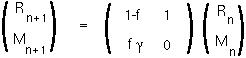
Solving Linear Equations: Red Blood Cell Production

To avoid having to take the matrix M to the t power, we will find the coordinate system in which which the transition matrix is a diagonal matrix.

Step 2: Find the two eigenvalues of the matrix:

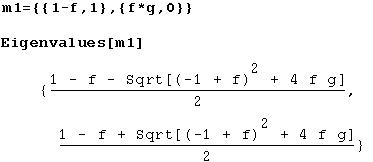
At this stage, let's consider the consequences of these eigenvalues.

If both of the eigenvalues are less than one in magnitude, then Dⁿ will go to zero over time. Since 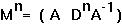, then Mⁿ must also go to zero, which tells us that R[n] and M[n] will go to zero and there will be no more blood cells in the body.

If at least one of the eigenvalues is greater than one in magnitude, then Dⁿ will grow over time and so Mⁿ will grow over time. [In fact, it will grow in the direction of the eigenvector associated with the eigenvalue that is greater than one.] But this means that the number of red blood cells in the body will grow continuously over time and eventually the body would pop.

Therefore, the only way for the total red blood cell count in the body to remain more or less constant is if the eigenvalue with the greatest magnitude (the leading eigenvalue) equals one.

From the equations for the eigenvalues, the leading eigenvalue will equal one only if equals one. We therefore assume that this is true.

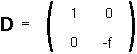
Then the eigenvalues will equal 1 and -f.

Solving Linear Equations: Red Blood Cell Production

We now proceed assuming that

=1.

Step 3: A diagonal matrix D which is similar to M is:

Step 4: Find the two eigenvectors of the matrix M:

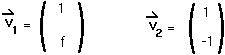
Step 5: Therefore the transformation matrix, A, is :

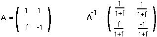
Matrix A changes the coordinate system to one in which the transition matrix is diagonal.

Solving Linear Equations: Red Blood Cell Production

Step 6: M to the n power is therefore equal to:

and we can write the general solution as:

In particular,

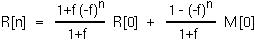
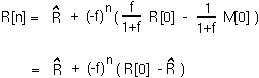
Since f is the fraction of RBCs removed be the spleen every day, we may assume that f lies between 0 and 1. Therefore, as n goes to infinity, R[n] will go towards the equilibrium value of (R[0]+M[0])/(1+f) = .

At this point, we can use the equilibrium value to write the equation in a much simpler form:

Solving Linear Equations: Red Blood Cell Production

We now draw several conclusions about the behavior of the system.

Firstly, the number of red blood cells will oscillate towards its equilibrium value (since -f is negative). This occurs because of the time delay inherent in the model: the bone marrow produces cells today in proportion to the number of cells that died yesterday.

Secondly, the approach to equilibrium will be rapid if f is small and the spleen filters out few cells everyday. I think that this is a very counterintuitive and suspect (!) result, since it implies that if the spleen works very slowly as a filter then the blood system will equilibrate faster.

Thirdly, there are a number of other unreasonable features about this model.

If you ever give blood, then R[n]+M[n] is reduced by the number of RBCs in a pint of blood and the total number of RBCs will always remain at this reduced value. That is, there is no homeostatic mechanism inherent in the model. If the total number of RBCs is perturbed for some reason, it will never go back.
How does the bone marrow know how many RBCs were filtered in the previous day?

It therefore seems like a good idea to scrap the model and start again.

Solving Linear Equations: Red Blood Cell Production

Lets simply change the assumption that the bone marrow makes cells in proportion to the number that were filtered out in the previous generation.

Instead, lets assume that the same number (c) of red blood cells are produced by the bone marrow every day.

We then get a simpler one-variable model:

R[n+1] = (1-f) R[n] + c

The equilibrium number of red blood cells will now equal c/f.

We can then write the recursion in terms of how far off the number of RBCs is from the equilibrium value:

(R[n+1]-c/f) = (1-f) R[n] + c - c/f = (1-f) (R[n]-c/f)

which can be easily iterated:

(R[n]-c/f) = (1-f)ⁿ (R[0]-c/f)

This model seems to behave much more realistically:

First, the system will equilibrate faster if f is large and the spleen filters out many cells (which makes more sense to me).
Secondly, if we perturb the number of RBCs (by donating blood for example), the number of red blood cells will eventually return to the same equilibrium (c/f). The system would be homeostatic.
Thirdly, we needn't assume any feedback loop between the spleen and the bone marrow. The bone marrow just produces a constant number of red blood cells every day.

This example illustrates the need to check the model and its results to see if they are reasonable and the need to scrap the model if they are not!

Back to biology 301 home page.