Methods of Analysis. IV. General Solutions

With some equations, we can determine the general solution which describes where the system will be at any time in the future.

General solutions are extremely useful because

• future states can be determined by plugging numbers into a single equation
• global (and not just local) stability properties can be determined.

Unfortunately, not all non-linear equations can be solved directly.

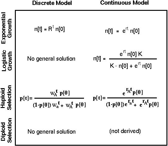
For instance, the diploid selection model in discrete time and the logistic model in discrete time do not have an explicit general solution.

Exponential Growth in Discrete Time

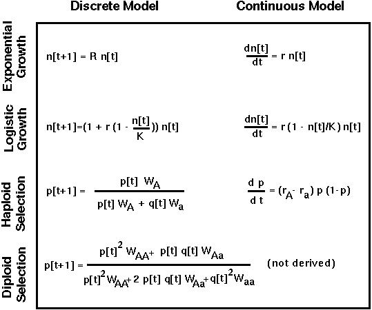
If R is the number of offspring per parent and if there are n[t] individuals in the population at time t, then in the next generation there will be:

Starting at generation 0, there will be R n[0] individuals in the first generation, R² n[0] individuals in the second generation, R³ n[0] individuals in the third generation, and so on.

n[t] = R^t n[0]

This is the general solution giving the population size over time.

Exponential Growth in Continuous Time

To solve this equation, perform a "separation of variables" and integrate both sides:

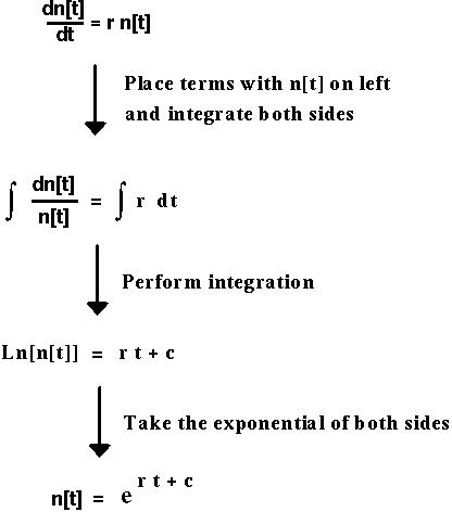
At time t=0, n[0] = Exp[r*0+c], which tells us that Exp[c] must equal n[0].

n[t] = Exp[r t] n[0]

Exp[r] plays the same role in the continuous time model as does R in the discrete time model.

Logistic Model (Discrete)

Logistic Model (Continuous)

Logistic Model (Continuous)

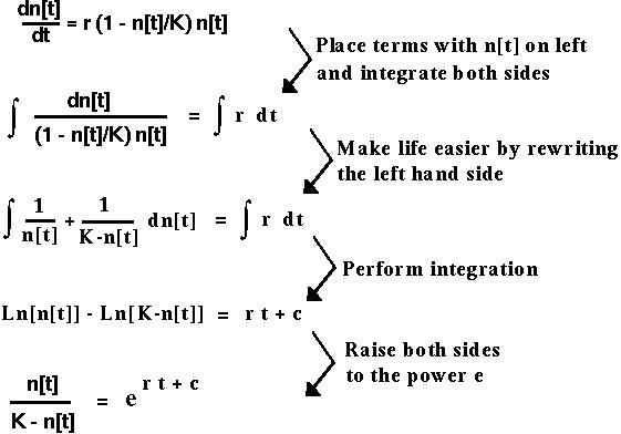
At time t=0, this equation reduces to n[0]/(K-n[0]) = Exp[c], which we can then use to replace Exp[c].

We then solve for n[t]:

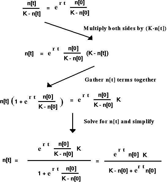
Does this make sense?

• At t=0, it does reduce to n[0].
• As t gets really large, if r is positive then n[t] approaches K.
• As t gets really large, if r is negative then n[t] approaches 0.

Haploid Selection Model (Discrete)

For discrete time models, one method that sometimes works is:

• write p[t] as a function of p[t-1]
• write each p[t-1] as a function of p[t-2]
• simplify

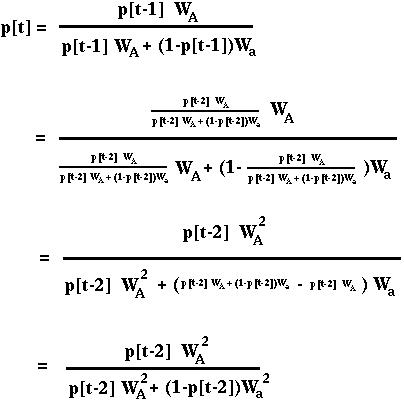
We could repeat these steps to write p[t] as a function of p[t-3]. The fitnesses would then be cubed rather than squared.

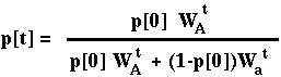
Repeating the method t times would give:

Haploid Selection Model (Discrete)

• let x[t] = p[t]/(1-p[t]), in which case, p[t] = ?
• let x[t] = p[t] - (often helpful when there is only one equilibrium)

In this model, the first transformation makes the equations much simpler:

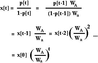
This tells us a bit more about how selection acts in the haploid model: the ratio of A to a alleles changes by a constant amount each generation!

To transform back into the original variable, note that p[t] = x[t]/(x[t]+1):

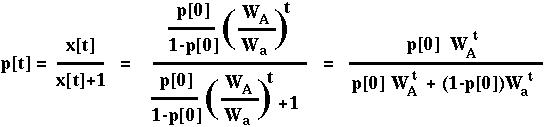
which is the same solution as we had above.

This general solution can be used, for example, to determine how much time it would take for a given change in the frequency of an allele.

Haploid Selection Model (Continuous)

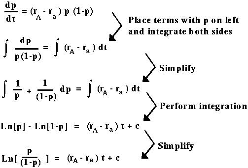
We then solve for p:

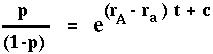
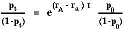
Finally, we plug in an initial condition. Say that at time t=0 the allele frequency is p₀. Then at time t the allele frequency, p_t will solve:

Again this tells us that the ratio of A to a alleles changes at a constant rate over time.

Haploid Selection Model (Continuous)

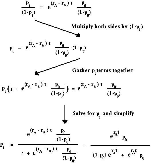
Exp[r_A] and Exp[r_a] in the continuous time model play the same role as W_A and W_a in the discrete time model.

The continuous time model exhibits the same behavior over time as the discrete time model.

Diploid Selection Model (Discrete)

Methods of Analysis. IV. General Solutions

Back to biology 301 home page.